Access Links

• 👨‍💻 Model & Code: yuk068/traffic-collision-anticipation-model
• 🎥 Video Demo: Youtube - Yuk
• ⌛ The project spanned from the middle of May, 2025 till around the end of May, 2025.

Prologue

This was my work for the MAT3562E - Computer Vision course at HUS-VNU. The story and motivation behind it was relatively similar to my project for the MAT3533 - Machine Learning course last semester, but also a fresh experience. And yeah, I’m the only second year in the class again.

So yeah this semester i signed up for computer vision, also looking to make a project like with machine learning. Its a longer story actually, originally for this semester (2nd semes of second year), I signed up for like 3 project driven courses, and was planning to tackle all of them with 1 project, at first I was thinking of multimodal AI because it ticks all the box for the courses, but, some stuff happened so this project was much more separate from anything LLM or NLP, I might talk about this semester more in some other post.

But anyway, this course, this project, was pretty decent. I was especially intrigued by the lecturer of the class, in this wackahh school, she actually seems genuinely passionate about her craft and her connection with the students. It almost feel like she is in the wrong place, much like me lol, but, i quite admire her, even if she didnt grade the project as high as the machine learning one.

This project, originally, I had much bigger ambition for it, but, due to time constraint and more, the end product is still acceptable for me.

Table of Content

Project Overview

So like I said, at first I was planning to do something with multimodal AI to use the computer vision section in it for this course, but, this project is pretty rooted in both computer vision and deep learning. With such a change of plan, I was scouring for some kind of problem to solve for the final project. Yuk being Yuk, I just wanted to really do something that has value and also learn as much as possible, so, I start checking out the recent competitions on Kaggle, and I came across 🚗💥 Nexar Dashcam Crash Prediction Challenge.

Nexar Dashcam Crash Prediction Challenge

The data consists of ~3,000 videos, divided into two groups: normal and with/near collisions. The training set includes 1,500 videos lasting 20-40 seconds, accompanied by timestamps for warnings and collisions, while the test set consists of shorter videos (~10 seconds) containing only the initial part before a potential collision.

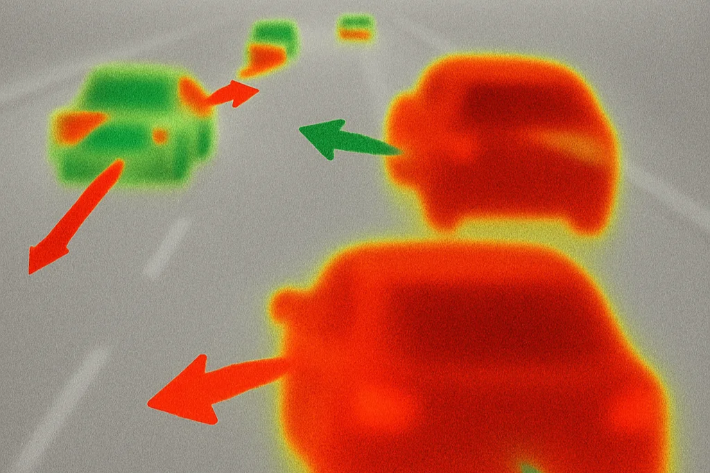
The goal of the competition was to create an Early Traffic Collision Anticipation model, this is different from Traffic Collision Prediction in that we have to be able to spot the risk in real time and give ample warning for the driver, not detecting a collision in post. So you dont just provide a risk score for a video, but you need a running risk score that is as relevant to the live POV of the driver as possible. This make it significantly more high-stake and harder from a technical stand point, but i liked it. You know when sitting in some cars, when a near collision is of risk it beeps like crazy? What I wanted to achieve was similar to that.

Another thing about the task is that we are only given dashcam footage and timestamp, so no extra sensory data, LIDAR, etc… This kinda makes it an ill-posed problem, but I had this implication: perhaps by just using dashcam footage, we are striving for a more experimental, incremental approach. To not only utilize the already vast amount of dashcam footage that might have not been annotated. Furthermore, this is a kind of application that is quick and easy to implement, dashcams are already almost a necessity in most vehicle, and it does not require any additional physical modification to the vehicle. But thats just my two cent.

Planned Methodologies

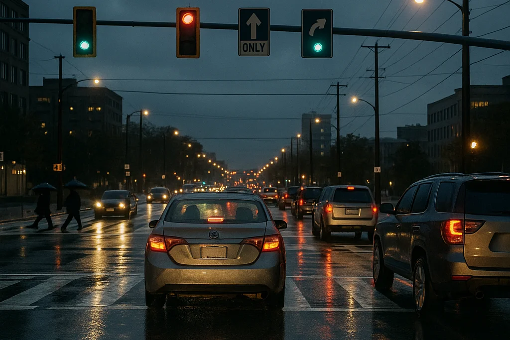
Anyway, the challenge immediately caught my eye, a real problem, dataset from a company, truly a step up from my machine learning project, so I took it up. After some researching, originally I planned to tackle 2 approach for the problem, for funsies I also generated two “thumbnail” for the two methods lol:

• M1 (Method 1): A more symbolic approach, using object detection and segmentation as the backbone. So we dont bother with things like what color is a car or road is and so on. In its simplest implementation that I could thought off, something like, use YOLO to segment cars, then estimate stuff like distance and motion, depth, and so on, and from there, maybe even somehow estimate speed, other aspect like traffic lights, weather, pedestrian, etc… All of which will be fed into a GNN (Graph Neural Network), which I believed was suitable for the kind of input we are talking about. Sadly, due to time constraint, I hadn’t actually explore this approach, so, I guess I’ll put a tack on this, what I did implement, is this project-method 2.
• M2 (Method 2): Global semantic approach, instead of focusing on subjects like M1, we take in everything, or less elegantly, just chuck it into the usual pretrained CNN lol. So yeah thats basically the gist of this approach, much more straightforward and conventional, definitely in the realm of “blackbox”, but worth trying nevertheless.

Long story short, exploring the M2 approach, I eventually crafted the model below:

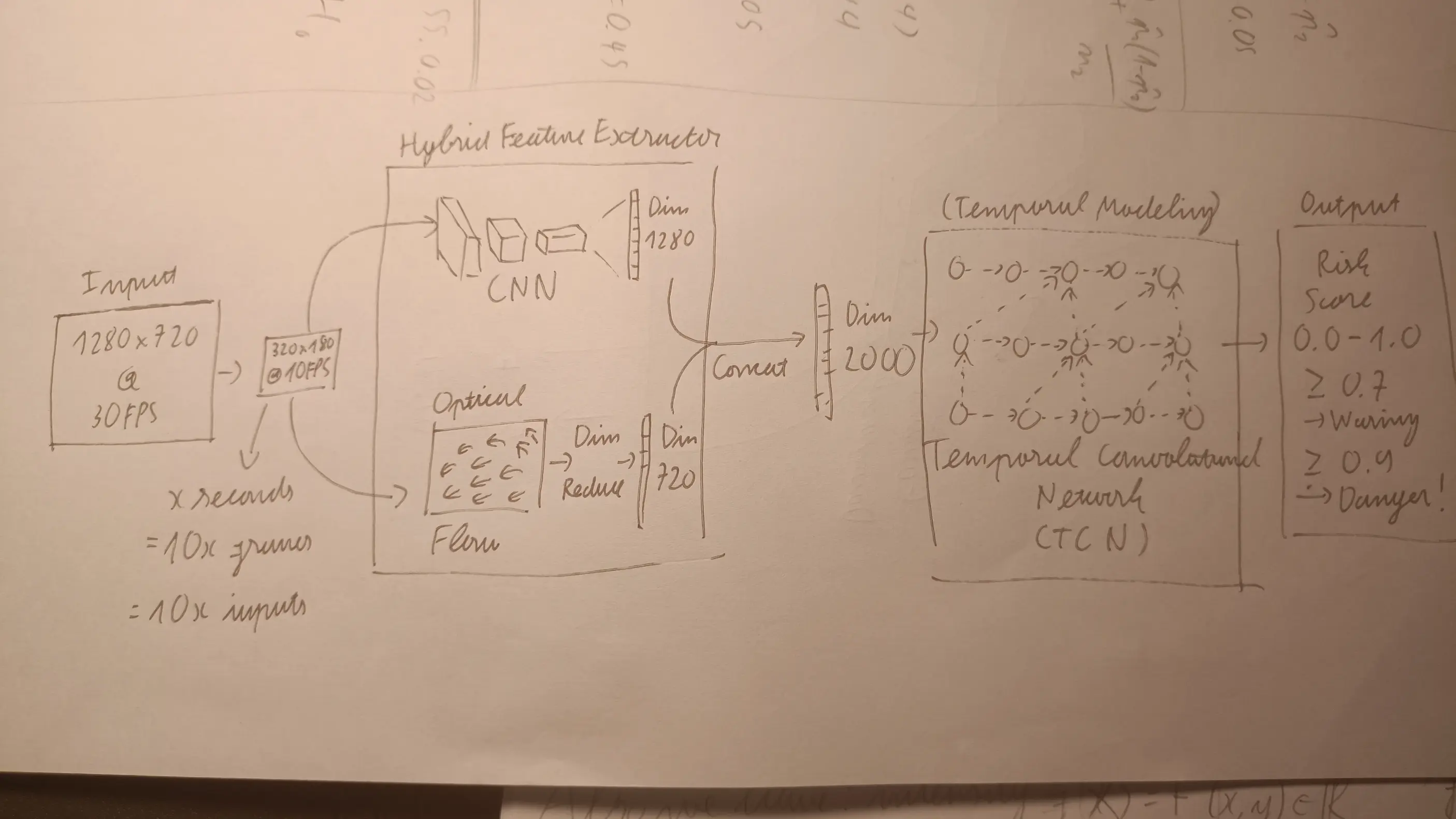
In general, the model is divided into two module:

• Hybrid Feature Extractor: Hope of achieving a comprehensive understanding or both image and motion, producing a rich feature vector for each frame.
  • CNN-backbone: EfficientNetB0
  • Motion input: Gunnar Farneback Optical Flow
• Temporal Convolutional Network (TCN): For temporal modeling, as prediction from a sequence of frames is definitely more feasible than one.

EfficientNetB0

EfficientNet is a family of pre-trained CNNs first introduced in Tan & Le., 2019, I’ve actually already covered the model that I used (EfficientNetB0) in this post: CNN Technical Breakdown: EfficientNetB0.

In short: CNN-backbone, similar to those pre-trained with ImageNet, used for the “Image Understanding” of this hybrid feature extractor. It produces 1280-length feature vector. I chose this one because it was relatively fast, capable of running on edge-devices, easy to work with, accessible too. Furthermore the original paper was co-authored by a Vietnamese so yeah.

Gunnar-Farneback Optical Flow

This is the “Motion Understanding” module of the hybrid feature extractor. I’m probably won’t go too deep into this algorithm and save it for like a separate post or maybe even a Youtube video because this thing is actually quite difficult to breakdown without visualization. In this section im just gonna show some math that ive written down.

Honestly, this is one of the most fascinating algorithm that I’ve ever come across, and it make me truly admire the man behind it-Gunnar Farneback, like how the hell did he came up with this??? This algorithm seems to be originally introduced in his paper: Farneback., 2003.

Also, there is very likely to be errors in the derivation, so I’d really appreciate any suggestion and correction in the comments, I highly advice you to double check the math should you follow this.

Optical Flow

Optical flow in this context, is the apparent motion of brightness patterns (intensity) in an image sequence, typically between two consecutive frames. It represents how each pixel in the first frame has moved to a new location in the second frame, encoded as a 2D displacement vector field. This motion estimation is foundational in understanding scene dynamics, object tracking, and video analysis.

In our case of 2 frame -> vector field, there are 3 main algorithms:

• Lucas-Kanade
• Horn-Schnuck
• Gunnar Farneback

We will cover the Gunnar Farneback algorithm in this section. Thus, we will formalize our input and output:

• Inputs:
  • Given frame 1: $ F_1 \in \mathbb{R}^{W \times H} $ as our starting image/frame of width $ W $ and height $ H $.
  • Given frame 2: $ F_2 \in \mathbb{R}^{W \times H} $ as the target frame of our motion estimation task.
• Output: Dense 2D vector flow field $ D \in \mathbb{R}^{W \times H \times 2} $.

Image Patches as Quadratic Polynomials

At the heart of the algorithm, Farneback introduced a brilliant idea: we estimate dense global motion by using local “patches”, its basically a $ p \times p $ area of an image, much like a filter/kernel in convolution just by mental image. But, if we are able to identify a patch by its brightness/intensity pattern, how would we know where it has moved in the image?

Lets just consider the simplest case, where the image is binary, ie. 0 intensity represent white and 1 intensity represent black (this algorithm works on grayscale image btw, so if we are estimating between two RGB images the algo will convert it to grayscale). Say with a $ 5 \times 5 $ patch, one way to figure whether it has moved or not is to scan the entire image to find that exact $ 5 \times 5 $ patch again, but obviously, this is impractical, and doesn’t make sense in an actual sequence say a robot arm monitoring system or dashcam footage.

So, Farneback’s solution? modeling each patch as a quadratic polynomial. Instead of intensity $ I(\mathbf{x}) $ where $ \mathbf{x} = (x, y) $ being just a single number (0/1, 0-255,…), we model this pixel in tandem with its local neighboring pixels as:

\[I(\mathbf{x}) \approx \mathbf{x} A \mathbf{x}^\top + b^\top \mathbf{x} + c\]

Where:

\(A = \begin{bmatrix} a_1 & a_3/2 \\ a_3/2 & a_2 \end{bmatrix}\) \(; \mathbf{b} = \begin{bmatrix} a_4 \\ a_5 \end{bmatrix}\) \(; c = a_6\)

Thus we have:

\[I(x, y) \approx a_1 x^2 + a_2 y^2 + a_3 x y + a_4 x + a_5 y + a_6\]

For the scope of this post, you can just assume intuition wise that this quadratic polynomial (QP) is enough to capture not only 1 pixel but also its neighboring region, thus, a pixel now is “identified” by not just its intensity but also its neighboring structure.

Fitting a QP to a pixel

Now that we have:

\[I(x, y) \approx a_1 x^2 + a_2 y^2 + a_3 x y + a_4 x + a_5 y + a_6\]

We can define:

\[\phi(x, y) = \begin{bmatrix} x^2 & xy & y^2 & x & y & 1 \end{bmatrix} \\[7pt] \mathbf{a} = \begin{bmatrix} a_1 & a_2 & a_3 & a_4 & a_5 & a_6 \end{bmatrix}\]

And get:

\[I(x, y) \approx \phi(x, y)^\top \mathbf{a}\]

Now, for a $ p \times p $ region, and $ n = p^2 $, we have:

\[\underbrace{ \begin{bmatrix} x_1^2 & y_1^2 & x_1 y_1 & x_1 & y_1 & 1 \\ x_2^2 & y_2^2 & x_2 y_2 & x_2 & y_2 & 1 \\ \vdots & \vdots & \vdots & \vdots & \vdots & \vdots \\ x_n^2 & y_n^2 & x_n y_n & x_n & y_n & 1 \\ \end{bmatrix} }_{\Phi \in \mathbb{R}^{n \times 6}} \underbrace{ \begin{bmatrix} a_1 \\ a_2 \\ a_3 \\ a_4 \\ a_5 \\ a_6 \end{bmatrix} }_{\mathbf{a} \in \mathbb{R}^6} = \underbrace{ \begin{bmatrix} I_1 \\ I_2 \\ \vdots \\ I_n \end{bmatrix} }_{\mathbf{I} \in \mathbb{R}^n}\]

Stacking this into a linear system, we get ourselves an overdetermined least squares problem:

\[\Phi \mathbf{a} = \mathbf{I}\]

We now can solve for the coefficients $ \mathbf{a} $ using Ordinary Least Squares (OLS):

\[\mathbf{a} = \left(\Phi^\top W \Phi \right)^{-1} \Phi^\top W \mathbf{I}\]

Where, for now, you can just assume $ W = I \in \mathbb{R}^{n \times 6} $ (identity). Similar to linear regression, this can either be solved by a closed form solution or iteratively (opencv implements iterative solver) And remember that:

\(A = \begin{bmatrix} a_1 & a_3/2 \\ a_3/2 & a_2 \end{bmatrix}\) \(; \mathbf{b} = \begin{bmatrix} a_4 \\ a_5 \end{bmatrix}\) \(; c = a_6\)

Thus, by solving for $ \mathbf{a} $ we will get our desired estimation via QP:

\[I(\mathbf{x}) \approx \mathbf{x} A \mathbf{x}^\top + b^\top \mathbf{x} + c\]

That represent a single pixel in relation to its local structure.

Estimating Motion between Image Patches

The assumption that enables the estimation of motion between 2 patches in the algorithm, is that the patches are still the same QP, just shifted slightly, formalizing this:

• Say we have two patches $ I_1 $ and $ I_2 $:

\[I_1(\mathbf{x}) \approx \mathbf{x} A_1 \mathbf{x}^\top + b_1^\top \mathbf{x} + c_1 \\ I_2(\mathbf{x}) \approx \mathbf{x} A_2 \mathbf{x}^\top + b_2^\top \mathbf{x} + c_2\]

\[I_2(\mathbf{x}) = I_1(\mathbf{x} - \mathbf{d}) = (\mathbf{x} - \mathbf{d}) A_1 (\mathbf{x} - \mathbf{d})^\top + b_1^\top (\mathbf{x} - \mathbf{d}) + c_1\]

Where by using a very strong assumption that $ A_1 = A_2 = A $ (it was hard for me to accept that too… you may do your research on why so far there are so many strong assumptions), then you can directly solve for $ \mathbf{d} $ using the closed form solution (derivation as an exercise to the reader lol):

\[\mathbf{d} = \frac{1}{2} A^{-1} (b_1 - b_2)\]

Thus, we get the vector $ \mathbf{d} \in \mathbb{R}^2 $ as the displacement vector between pixels-represented-by-patch $ I_1 $ and $ I_2 $. Do this for the entire image, and we will get the dense vector field $ D \in \mathbb{R}^{W \times H \times 2} $.

Note: $ I_1 $ and $ I_2 $ represent THE SAME pixel in two frames, we are NOT looking for $ I_1 $ in frame 2 by scanning the image or something.

The Pyramid Strategy

If you are following this, you may wonder, with all these assumptions, how the hell can these premises even track motion by as little as a single pixel shift between 2 frames? This is where, the Pyramid Strategy comes in. Im now going to guide you through a mental model that helps to visualize this so called pyramid, Ill also include an illustration for clarity (yeah this is the part that is much more easily explained with a video):

Imagine the frames that you got, there are 2 of them, both of size $ W \times H \times 1 $ (grayscale), now stack them on top of eachother, this is the base for our pyramid, also called layer $ L_0 $.

Now, use Gaussian blur to downsample both frames, say by a factor of two, now, at layer $ L_1 $ of our pyramid, we got 2 frames that are of size $ W/2 \times H/2 \times 1 $.

Repeat this until some arbitrary $ L_k $ layer, if the factor was instead some arbitrary $ z $ where the size of the two frames are now $ W/z^k \times H/z^k \times 1 $.

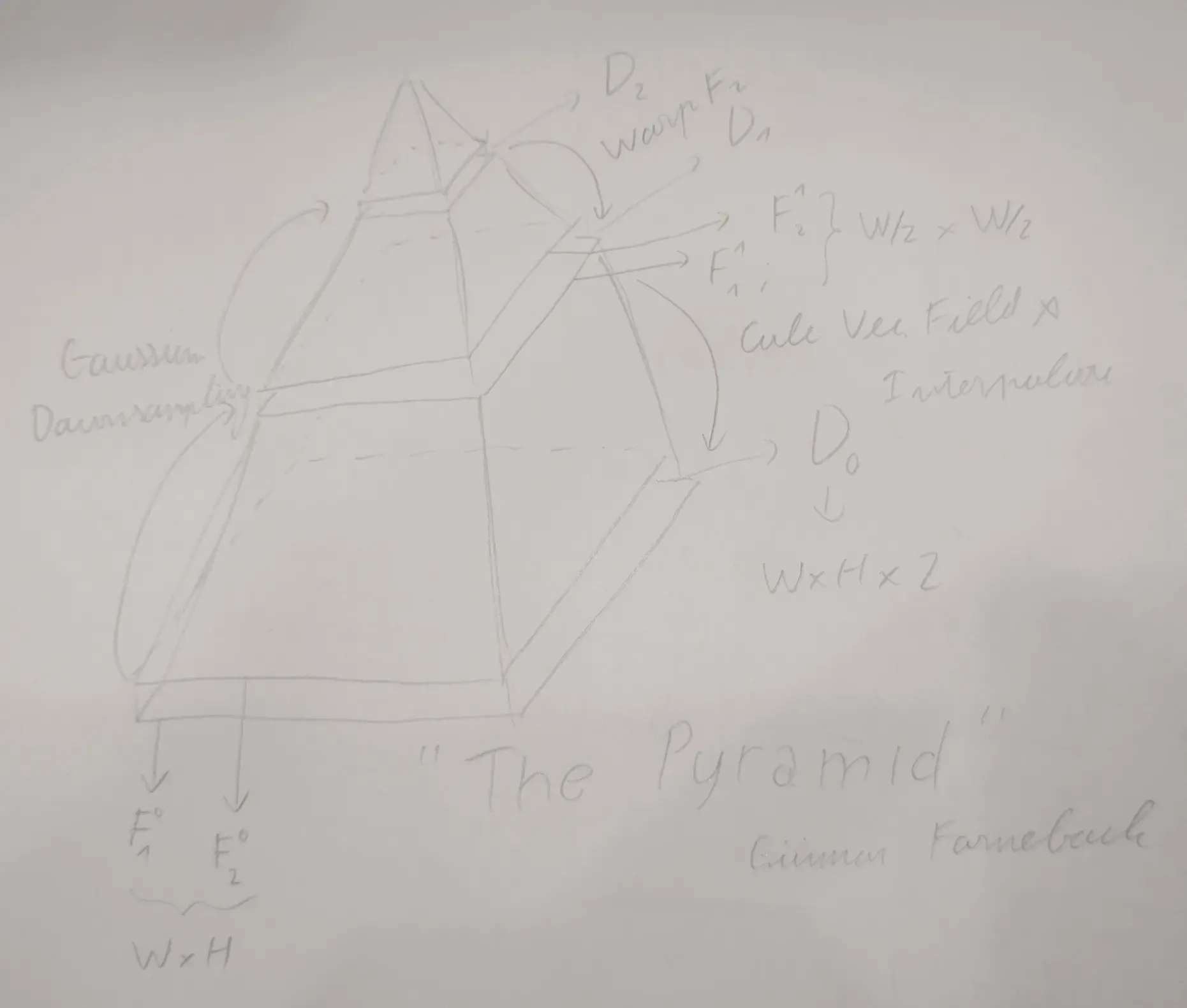
Now, we will work our way down from layer $ L_k $, because we will have frame $ F_k^1 $ and frame $ F_k^2 $ denoting the two frames at layer $ L_k $, we can solve for our first vector field $ D_k $, which will be of size $ W/z^k \times H/z^k \times 2 $

And, now that we have our first vector field $ D_k $, we will use it to “warp” frame $ F_{k-1}^2 $. In $ D_k $, define $ D_k(\mathbf{x}) = d_k(x, y) = (u, v) $ which is the motion vector at pixel positioned at $ x $ and $ y $:

\[\text{warped}\left(I_k^2(x, y)\right) = I_k^2(x + u, y + v)\]

Note that we are going to need some interpolation because $ x + u $ and $ y + v $ might not be ints. After getting this new warped second frame, we continue to solve for $ D_{k - 1} $, and work out way until $ k = 0 $, obtaining $ D_0 $, our vector field describing the motion between frame $ F_1 $ and frame $ F_2 $.

I get that this in genuinely pretty hard to grasp, so I don’t really expect you to get it on the first try, and that this derivation isnt really rigorous anyway, so im just gonna put some bullet points:

• The pyramid is what makes the Farneback algorithm practical, its fascinating, its like he came up with 2 algorithm with 1, 1 algorithm that has 2.
• The higher the layer, the more “abstracted” the movement are between two frames, so you may interpret that vector fields at those level describe more global motion.
• We warp the second frame with a prior vector field to somewhat compensate for the fact that the algorithm assumes very small motion, so with the pyramid, even when motion are big (eg. like a quick swipe from a turk, a turn from a car) we can still estimate them.

I truly suggest you look further into this algorithm, again, I appreciate any suggestion and correction. This small section really doesnt do this algorithm justice.

Hybrid Feature Extractor

Now that we have broken down the technical details of the two component in the hybrid feature extractor, do note that, the first component-the CNN, produces 1280 size feature vector. But, for the motion part, $ W \times H \times 2 $ (in this case 320x180x2) was obviously way too many values, so I basically divided the vector field into equally sized grids, and “summarized” the motion in that grid with statistics, dominant component, and so on, eventually reducing the motion information to a 720 size feature vector.

Concatenating the two feature vector, image and motion, gives us a 2000 size rich feature vector, for each frame, ready to be put through the next module-temporal modeling.

Temporal Convolutional Network (TCN)

After we got our hybrid feature extractor, now each frame (or frame-pair) will get a rich representation that captures both Image and Motion understanding, comes our next step in the pipeline: Temporal Modeling.

At first, because we already have feature vector for each frame, and we can even stack them to form a [batch_size, sequence_length, num_features], I immediately think of recurrent models, like LSTM and GRU, however:

• They are too slow for real time processing, can’t be parallelized.
• They are quite notorious for being hard to train.

So after some extra researching, I stumbled upon a network that ive never heard of before: Temporal Convolutional Network (TCN), which was first introduced in Oord et al., 2016. Which essentially solved all the problems that I had with recurrent models. Im not really feeling like going deep into this model, Imma be real its not exactly a perfect fit for the task and I didnt really utilize it fully, so for another day I guess.

Anyway, I chose the sequence length to be 2 seconds, which equates to 20 frames, each with a feature vector of size 2000, making it [batch_size, 20, 2000], to output a single risk score. Again, due to time constraint, the training was quite half-assed and I believe the fact that I didnt do much with the data contributed to the limitation of this project.

“Final” Product

At this point the deadline was closing in so I just trained and it was actually kinda fine, definitely not up to my standard for a task so high-stake, but presentable for the finals at least.

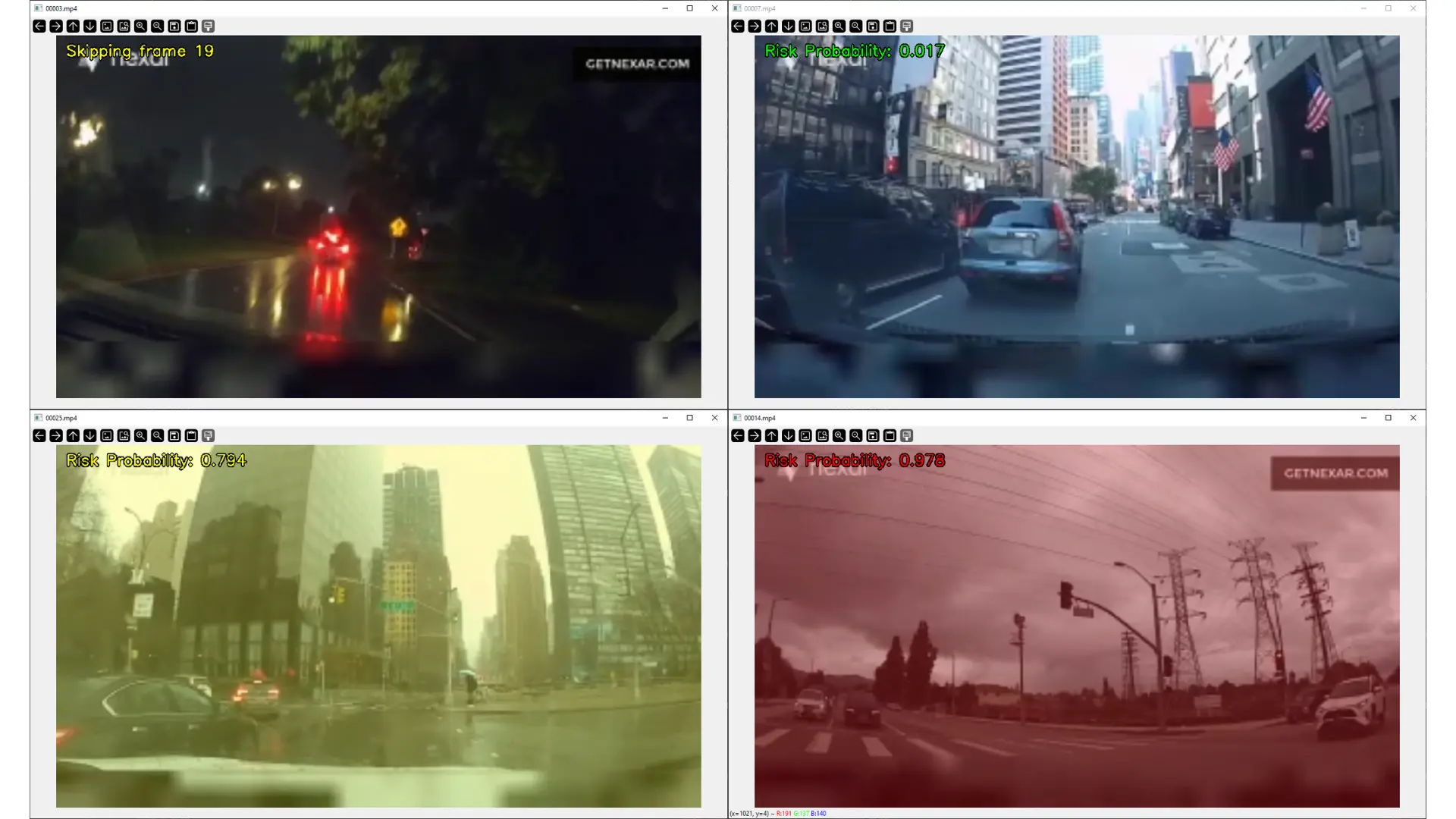
You may watch the demo here: Youtube - Yuk.

Epilogue

So yeah, if you haven’t already noticed I’m not exactly that excited with this project anymore. Mostly because that for me, computer vision is often more trivial than NLP lol. Like nowadays to solve any CV task you essentially have a plethora of tools in the box already, and I do think vision models are generally more robust than LLMs, especially when taking model size into account. Another reason is because right now, as of writing this, I’m aiming for a job that is much more oriented to NLP, but, I still wanted to write about this project, I had been postponing it anyway.

Who knows, maybe, one day I’ll pick up this project again, and explore that M1 that is still very intriguing to me. Perhaps this could have been more than what it is now had it not been tied to the span of the course. But, yeah, I think I did my best, I tackled something new, learned a ton of new stuff, and, had a presentable demo.

I think my biggest fascination when it comes to computer vision, is to eventually work on some kind of vision system for robotics, or maybe even to contribute towards the recent research on world models like V-JEPA, so yeah, I definitely don’t “dislike” CV, its just that I do think a lot of its simplest problems are as saturated as web dev projects (though lets be fair, LLMs are getting to that level as well).

Thanks for reading through this, Ive just been trying to finish these up in like less than a day, so its sloppy I know, but, i do feel good that I still did it, until next time.