Paper Comprehension: Motion Planning Transformers
Prologue
This post is the continuation of Paper Comprehension: Motion Planning Networks.
From my understanding, Motion Planning Transformer (MPT) actually differs quite a lot from Motion Planning Network (MPNet) (and much more complicated too, which is to be expected). Nevertheless, the MPT paper authors does include the first author of the MPNet paper, professor Ahmed H. Qureshi.
So in this post, I’m going to breakdown the paper Motion Planning Transformers: A Motion Planning Framework for Mobile Robots, Johnson et al,. 2022. And give my final thoughts for both MPNet and MPT at the end.
Table of Content
Block
- Reference: Motion Planning Transformers: A Motion Planning Framework for Mobile Robots, Johnson et al,. 2022
1. Recap
The MPT module is a region proposal network that uses a transformer network to identify regions of interest, this region is then utilize by classic sampling-based motion planning methods (SMP), significantly reducing the search space and time in their testings.
Here is a quick comparison between MPT and MPNet:
| Model | MPT | MPNet |
|---|---|---|
| Architecture | Transformer (Encoder only) + Classifier (1x1 Conv) | CAE + DNN |
| Inference | Search region proposal | Autoregressive path generation |
| Map size | Handle variable sized maps | Can’t handle variable sized maps |
| Robot modality | Extends to and tested non-holonomic robots | Didn’t test with non-holonomic robots (in the specified paper, Baxter robot’s arm is still considered holonomic in its workspace) |
| Obstacle inputs | 2D Occupancy matrix (discretization if needed) | Point cloud coordinates as vector list (“hollow” obstacles) |
They tested their framework mostly in 2D space, including a point-mass case in $\mathbb{R}^2$ and a Dubins car case in $SE(2)$.
About problem definition, its essentially the same as the MPNet post so I won’t be going over it again, only difference is that our state can also be in $SE(2)$ space.
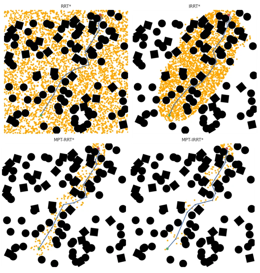
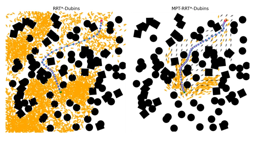
Fig. 1. and Fig. 2. Johnson et al,. 2022.
Overview of MPT Module for planning in $\mathbb{R}^2$.
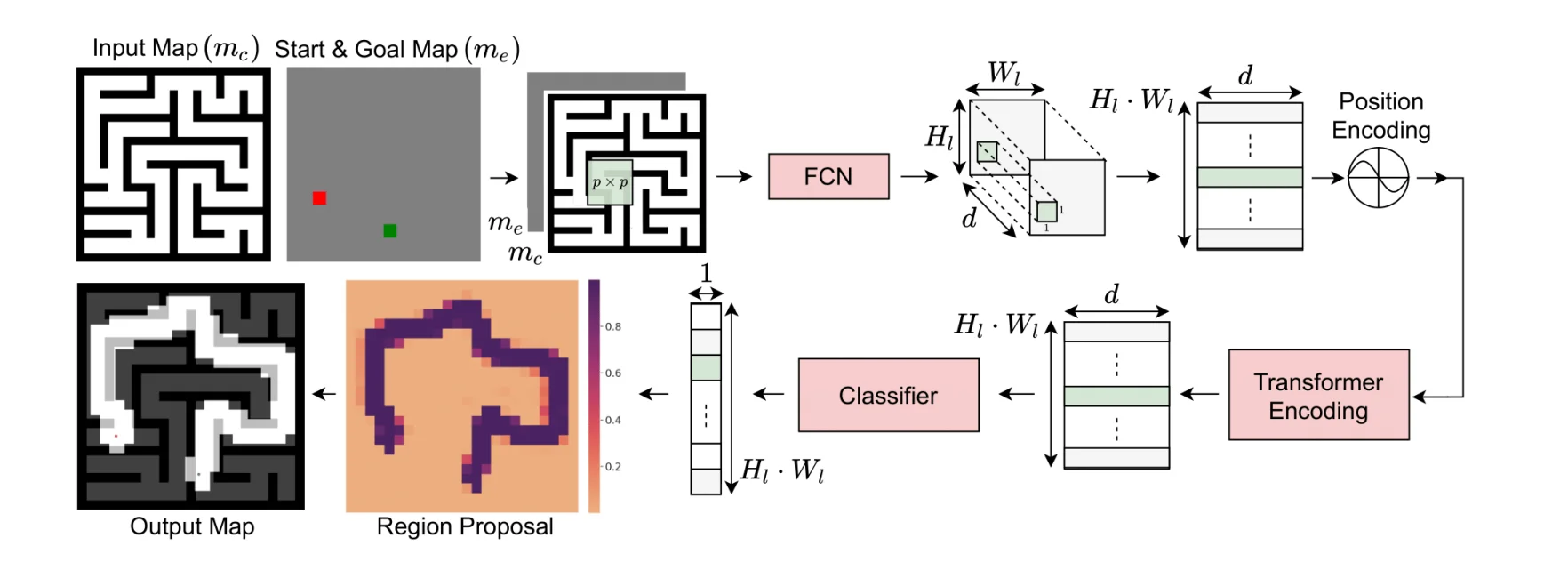
Fig. 3. Johnson et al,. 2022.
2. Architecture
2.1. Overview
The architecture of MPT is as follow, consider the point-mass robot case, in other words: state $x \in \mathbb{R}^2$.
Lets take the maze workspace of size $H \times W$ as an example here, the input to MPT will be $H \times W \times 2$. The second map is the “start-goal encoding map”, where the start and goal region will be encoded with a matrix of size $p \times p$ with -1 and 1, respectively.
These 2 maps will be concatenated to tensor $m$, and fed into the FCN network, where each patch will be convoluted with a sliding window of size $p \times p \times 2$, and after passing through ReLU and Maxpool Layers, we will get a new tensor of size $H_l \times W_l \times d$, lets call it tensor $M$.
Tensor $M$ is then flatten into a vector list of size $(H_l \cdot W_l) \times d$. Each patch will be “anchored” using the following indexing formula:
For each $(i_F, j_F)$ -th element in $M$ will be converted into index $j$ of the flatten list:
This vector list is will now be prepared as input for an Encoder block of the transformer, thus they will go through positional encoding, just like transformer for language modeling.
The Encoder includes components just like Vaswani et al,. 2017. Comprising of Multi-headed Self Attention block, Layer Norm, and residual connections. Dropout is also applied during training.
Passing through the encoder return us a new vector list of same size $(H_l \cdot W_l) \times d$. This vector list is then reshaped into a tensor $M’$.
Tensor $M’$ will then pass through a classifier (implemented as a 1x1 convolutional layer with Sigmoid activation) and give us output of size $H_l \times W_l \times 1$ , where each of these patch have activation $> 0.5$, we will highlight it as the “proposed region” of the MPT, finally giving us the masked output of size $H \times W$.
2.2. Positional Encoding
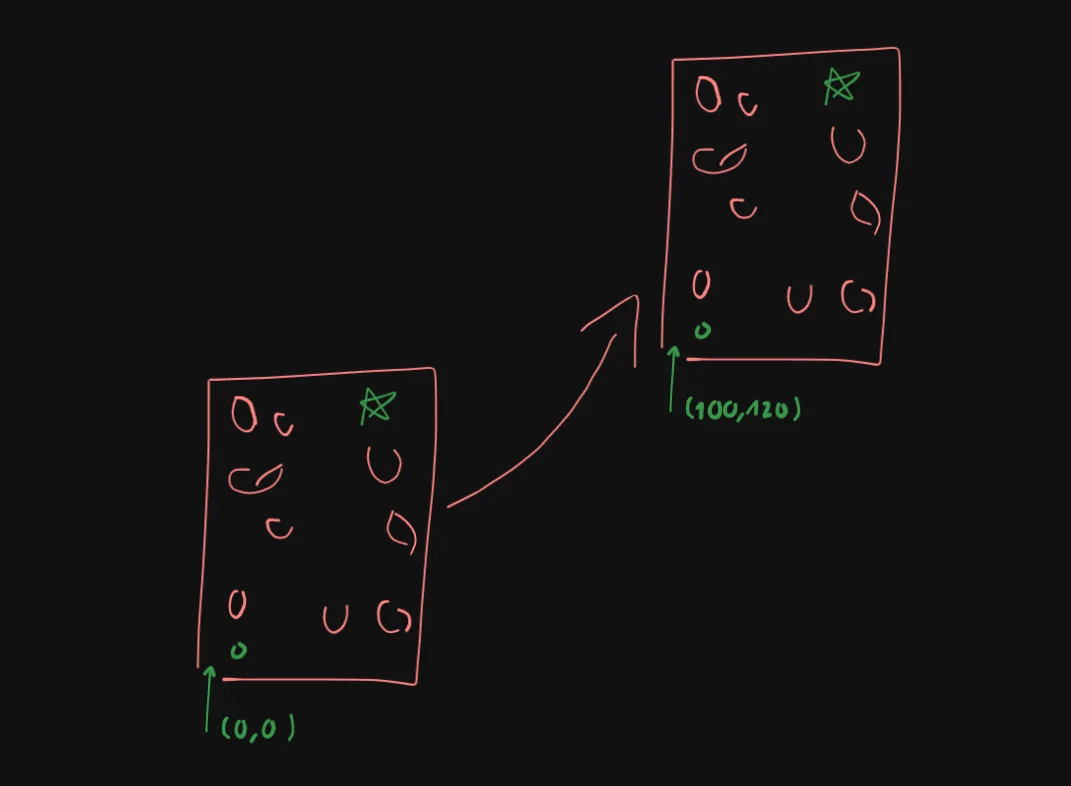
To ensure generalization to variable map sizes without having to generate training data of variable map sizes, the authors utilized Randomized Positional Encoding. Where beside the classic PE functions:
They randomly offsets and modify index $j$ to a new value.
To more easily visualize this, imagine we are on an infinite flat plane, and we put our finite map on this plane, naturally, the bottom left corner will usually be the origin $(0,0)$. And then we offset this entire map such that this origin becomes say $(100,120)$, and the more varies this is, the better chances that it will have seen coordinates outside of its initial map-bounded range.
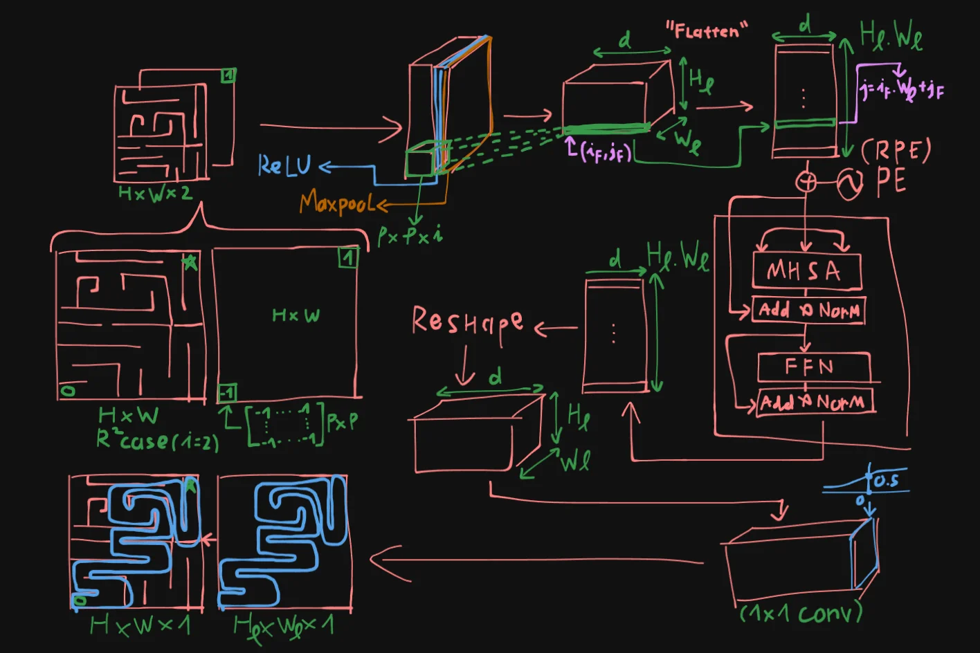
2.3. Extending to SE(2)
The way the authors extended this framework to say $SE(2)$, is demonstrated below:
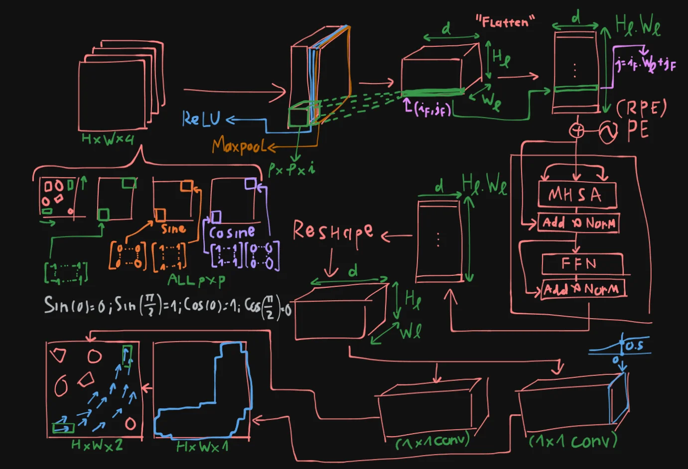
Essentially, instead of 2 input maps, they increase it to 4, where we have 2 additional Cosine and Sine maps that encodes the orientation of the start and goal positions.
In the diagram above you can see an example of what the input in the $SE(2)$ case might look like.
The bulk of the inference remains the same, except for the final output, where tensor $M’$ is passed through two separate classifier at the same time.
The first classifier still predicts a masked map, like the point-mass case, with Sigmoid activation and trained with cross-entropy loss.
The second classifier however, will predict an orientation map, in $SE(2)$, this is essentially a 2D vector field. This classifier does not have non-linear activation, instead, they train it to maximize cosine similarity with the target orientation map.
And then, only vectors that lies on the un-masked region will be kept, guiding the search.
2.4. Classical Planner
After the we have the proposed region by the MPT module, classical SMP methods can then utilize this region to search more efficiently. In case where the goal doesn’t lie in this region, we can explore the region outside the proposed map to ensure a feasible path is not overlooked.
3. Training
3.1. Rig, Loss, Optimizer
The authors trained MPT in an end-to-end supervised fashion. Each mini-batch was constructed from a single planning problem containing both positive and negative anchor points sampled from the environment map.
Training was performed using cross-entropy loss for anchor point classification together with cosine similarity loss for orientation prediction in the Dubins Car setting. The network was optimized using the Adam optimizer with $\beta_1 = 0.9$, $\beta_2 = 0.98$, and $\epsilon = 10^{-9}$. They additionally used the transformer learning rate scheduling strategy with 3200 warm-up steps.
All models were trained for 100 epochs with a batch size of 128 on a machine equipped with four NVIDIA RTX 2080 GPUs. The Point Robot model required approximately 21 hours of training, while the Dubins Car model required roughly 12 hours.
3.2. Data Generation
The authors generated training data separately for the Point Robot and Dubins Car environments across two workspace categories: Random Forest and Maze environments.
The Random Forest environment consisted of randomly placed circular and square obstacles, producing cluttered scenes with narrow passages. In contrast, the Maze environment was generated using randomized depth-first search, resulting in long-horizon planning problems where geometrically close start and goal states could still require highly circuitous trajectories.
For the Point Robot experiments, they generated 1750 maps for each environment category. On every map, 25 trajectories were collected using RRT*, with each planning query limited to a maximum runtime of 90 seconds.
For the Dubins Car experiments, they generated 900 maps from the Random Forest environment only. Similar to the Point Robot setup, they collected 25 trajectories per map using RRT*, but replaced the standard node connector with Dubins curves to satisfy non-holonomic motion constraints.
All occupancy maps used during training had a resolution of $(480 \times 480)$.
3.3. Negative Sampling
The training procedure relied on anchor point classification around expert trajectories. Anchor points located within 0.7 meters of a trajectory were treated as positive samples, while all remaining points were treated as negative samples.
To balance the training distribution, the authors randomly sampled negative anchor points using a 1:1 ratio between positive and negative samples. For the Dubins Car setting, each positive anchor point additionally stored an orientation label computed from the average trajectory orientation within the local neighborhood around the anchor point.
This formulation allowed the network to jointly learn trajectory occupancy likelihood and local motion direction from expert-generated paths.
4. Experiments & Results
4.1. Point-mass Robot
The authors evaluated MPT-aided planners against both traditional sampling-based planners and prior learning-based approaches on the Point Robot task. Their comparisons included RRT, Informed-RRT (IRRT), BIT, MPNet, NEXT-KS, and UNet-assisted planning variants.
The evaluation was conducted on 2500 random start-goal pairs sampled from the Random Forest and Maze environments. They reported three primary metrics: planning accuracy, planning time, and the number of sampled vertices used to construct the planning tree.
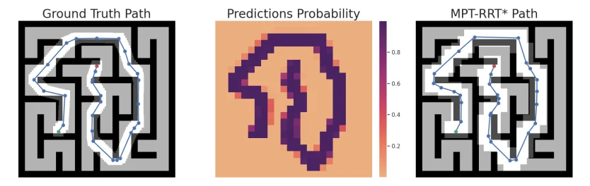
Fig. 4. Planned path for the Maze environment. Left: Ground truth path for a given start (green) and goal (red) point from the validation data. Center: The prediction probability from the MPT. Right: Masked map and planned trajectory for the given start (green) and goal (red) point using MPT-RRT*. Johnson et al,. 2022.
| Algorithm | Accuracy | Time (sec) | Vertices |
|---|---|---|---|
| rrt* | 100% | 5.448 | 3228 |
| irrt* | 100% | 0.425 | 267 |
| bit* | 100% | 0.477 | 819 |
| unet-rrt* | 30.27% | 0.167 | 168 |
| unet-rrt*-ee | 100% | 2.58 | 1913 |
| mpnet | 92.35% | 0.296 | 63 |
| mpt-rrt* (theirs) | 99.40% | 0.194 | 233 |
| mpt-irrt* (theirs) | 99.40% | 0.087 | 136 |
| mpt-rrt*-ee (theirs) | 100% | 0.211 | 247 |
Table I: Random forest environments, comparing planning accuracy, median time, and vertices on unseen environments. Johnson et al,. 2022.
| Algorithm | Accuracy | Time (sec) | Vertices |
|---|---|---|---|
| rrt* | 100% | 5.364 | 2042 |
| irrt* | 100% | 3.139 | 1394 |
| bit* | 100% | 2.870 | 2002 |
| unet-rrt* | 21.4% | 0.346 | 277 |
| unet-rrt*-ee | 100% | 4.133 | 2139 |
| mpnet | 71.76% | 1.727 | 1409 |
| next-ks | 28.27% | 3.021 | 387 |
| mpt-rrt* (theirs) | 99.16% | 0.870 | 626 |
| mpt-irrt* (theirs) | 99.16% | 0.784 | 566 |
| mpt-rrt*-ee (theirs) | 100% | 0.869 | 585 |
Table II: Maze environments, comparing planning accuracy, median time, and vertices on unseen environments. Johnson et al,. 2022.
Across both environments, the MPT-aided planners consistently reduced planning time and planning tree size relative to traditional planners. The improvement was particularly noticeable in the Maze environment, where long-horizon planning made geometric heuristics less effective. While IRRT* and BIT* achieved competitive performance in the Random Forest setting, their efficiency degraded in maze-like environments where the feasible path deviated substantially from the straight-line connection between start and goal states.
The authors further analyzed the distribution of planning time and sampled vertices using letter-value plots.
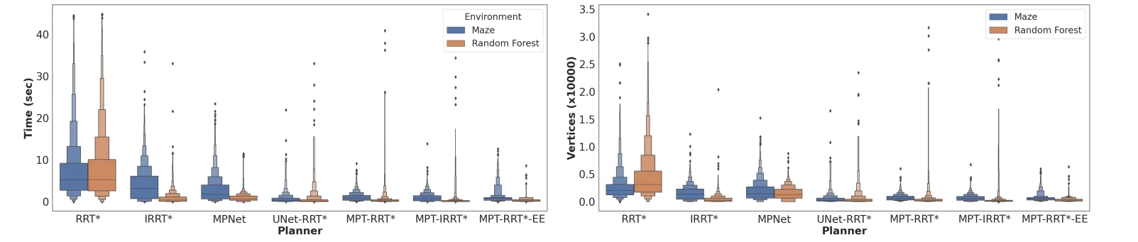
Fig. 5. Planning statistics for the Point Robot Model. Left: The planning time for traditional and learning-based planners. Right: Number of vertices in the planning tree for traditional and learning-based planners. MPT aided planners consistently reduce the planning time and the vertices in the planning tree, resulting in a lower variance of these statistics for these planners. Johnson et al,. 2022.
They observed that vanilla RRT* produced heavier-tailed planning distributions, especially for distant start-goal pairs that required denser exploration. In contrast, MPT-aided planners restricted exploration to regions highlighted by the transformer model, resulting in lower variance and fewer sampled states.
The paper also compared MPT against learning-based baselines such as UNet-assisted planning and MPNet. The UNet-based methods performed poorly, particularly in maze environments, which the authors attributed to the limited global reasoning capability of convolutional architectures. MPNet generalized better than UNet-based approaches, but still underperformed relative to MPT. The authors suggest that this gap may partially stem from differences in training scale, noting that MPNet was originally trained with substantially larger trajectory datasets.
To address occasional segmentation failures, they introduced an exploration-exploitation variant referred to as MPT-RRT*-EE. This hybrid strategy allowed the planner to occasionally sample outside the predicted region, recovering failed cases without significantly increasing planning cost. Using this approach, they achieved near-perfect planning accuracy while preserving low planning time and vertex counts.
The authors additionally evaluated generalization to unseen map sizes without retraining or fine-tuning.
| Map Size (# Obstacles) | Metric | RRT* | IRRT* | BIT* | MPT-RRT* | MPT-IRRT* | MPT-RRT* (F.E.) | MPT-IRRT* (F.E.) | MPT-RRT*-EE |
|---|---|---|---|---|---|---|---|---|---|
| 360×240 | Accuracy | 100% | 100% | 100% | 97.4% | 97.4% | 99.20% | 99.20% | 100% |
| (35) | Time (sec) | 5.926 | 0.286 | 0.625 | 0.265 | 0.062 | 0.248 | 0.054 | 0.297 |
| Vertices | 3660 | 257 | 1069 | 377 | 118 | 354 | 106 | 382 | |
| 480×240 | Accuracy | 100% | 100% | 100% | 96.3% | 96.3% | 98.5% | 98.5% | 100% |
| (50) | Time (sec) | 6.308 | 0.394 | 0.590 | 0.268 | 0.072 | 0.265 | 0.073 | 0.302 |
| Vertices | 3480 | 291 | 1061 | 348 | 130 | 319 | 131 | 362 | |
| 560×560 | Accuracy | 100% | 100% | 100% | 75.6% | 75.6% | 99.7% | 99.7% | 100% |
| (100) | Time (sec) | 6.725 | 0.283 | 0.397 | 0.253 | 0.082 | 0.181 | 0.083 | 0.217 |
| Vertices | 3854 | 203 | 810 | 262 | 101 | 218 | 112 | 237 | |
| 780×780 | Accuracy | 100% | 100% | 100% | 37.9% | 37.9% | 99.5% | 99.5% | 100% |
| (200) | Time (sec) | 8.095 | 0.476 | 0.542 | 0.274 | 0.095 | 0.297 | 0.152 | 0.285 |
| Vertices | 4292 | 255 | 974 | 284 | 142 | 241 | 161 | 238 |
Table III: Planning Performance Across Different Map Sizes, comparing planning accuracy, median time, and vertices for point robot on maps of different sizes. Johnson et al,. 2022.
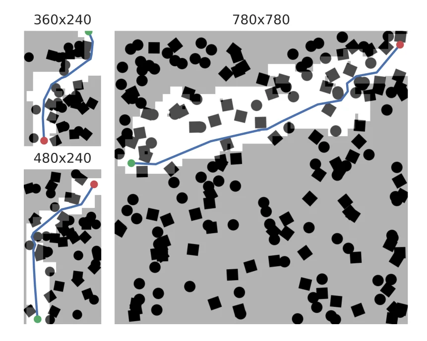
Fig. 6. Plot of paths for Random Forest environments of different size. The architecture of the MPT Model allows flexibility in planning for environments of different sizes. Johnson et al,. 2022.
They tested the same trained model on multiple map resolutions while maintaining obstacle density. Their results showed that MPT-aided planners retained low planning time and low vertex counts even as the search space increased. They also reported that randomized positional encoding substantially improved scalability compared to fixed positional encoding, particularly on larger maps.
4.2. Dubins Car
The authors further evaluated MPT on a non-holonomic Dubins Car model with state space $SE(2)$. In this setting, they compared MPT-assisted planning against RRT* and SST planners.
For geometric planning, Dubins curves were used as edge connectors, while SST generated trajectories through forward propagation of steering and velocity controls.
| Planner | Accuracy | Time (sec) | Vertices |
|---|---|---|---|
| Rrt* | 100% | 0.357 | 95 |
| Sst | 100% | 4.880 | 710 |
| Mpt-Rrt* | 95.15% | 0.176 | 59 |
| Mpt-Rrt*-Ee | 100% | 0.197 | 60 |
Table IV: Dubins Car Model Results, comparing planning accuracy, median time, and vertices for Dubins Car model for the Random Forest environment. Johnson et al,. 2022.
The reported metrics remained the same as the Point Robot experiments: planning accuracy, planning time, and number of sampled vertices.
Their results showed that MPT-aided planners reduced both planning time and sampled states relative to standard RRT*. The hybrid exploration-exploitation variant again achieved full planning accuracy while maintaining nearly identical computational cost.
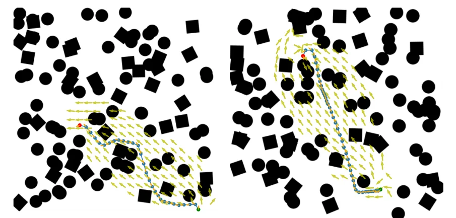
Fig. 7. MPT can also be trained to aid SMP planners for non-holonomic robots. Left and Right: Planned paths on Random Forest environment using MPT-RRT*. MPT identifies regions in $SE(2)$ through which a non-holonomic path exists. Johnson et al,. 2022.
The qualitative examples demonstrate that the transformer model was capable of predicting feasible regions within $SE(2)$, allowing the planner to focus sampling around kinematically valid corridors. By restricting exploration to these regions, the planner generated feasible trajectories using substantially fewer samples than the unaided planner.
The authors also observed that SST required significantly more samples and execution time, particularly in narrow sections of the environment where kinodynamic constraints complicated exploration.
5. Final Thoughts
5.1. MPNet vs. MPT
Looking back at both MPNet (2019) and MPT (2022), it is interesting to see the paradigm shift in just three years.
MPNet tried to tackle the problem head-on by autoregressively predicting the exact next state. While quite fast during inference, it struggled with generalization across diverse workspaces and required massive datasets for specific kinematics.
MPT took a different route: instead of forcing the network to explicitly draw the path, it used a Transformer to act as an “attention guide” for classical algorithms (like RRT*). This hybrid approach neatly bypasses the strict safety and feasibility guarantees that pure neural networks notoriously fail at.
However, MPT is not without its operational costs. While the authors state the inference is theoretically constant time, they do not explicitly disclose the parameter counts. Transformers are computationally heavy, and the self-attention mechanism scales quadratically with sequence length.
If one were to extend MPT to a 7-DOF robot like Baxter, discretizing a 7D space into just 10 segments per dimension results in 10 million grid cells. Suddenly, the region proposal becomes computationally intractable. MPNet at least avoided this specific grid bottleneck by taking raw point cloud vectors as input.
5.2. Peeking into 2026: Mobile Manipulators & Foundation Models
As you can see right now im busy with these foundational papers, I am just starting to map out the state-of-the-art in 2026. From recent literature, the landscape seems to have shifted heavily toward mobile manipulation, meaning robots are no longer just bolted to a pedestal (like Baxter) but are mounted on a moving chassis, or possess full humanoid mobility in $SE(3)$ space.
Motion planning for these systems introduces a complex challenge: the coupling of base and arm dynamics. You are planning for an omnidirectional base and the 7-DOF arm(s) simultaneously.
While older systems relied on a “Stop-and-Grasp” strategy, current research is pushing for “Grasping-on-the-Move,” where the base is in continuous motion while the arm executes the task.
To handle this complexity, the field appears to be moving beyond training isolated spatial networks. The new baseline involves Vision-Language-Action (VLA) foundation models, such as recent Gemini Robotics integrations. These models inherit semantic understanding from internet-scale pretraining. This allows them to process natural language inputs alongside RGB-D data, outputting discretized end-effector actions while handling emergent reasoning.
Despite the push toward these massive models, the industry standard for physical control strongly validates MPT’s core philosophy: the hybrid stack. End-to-end neural networks are rarely trusted blindly with physical hardware in shared human workspaces. Today’s systems use the VLA model for high-level semantic reasoning and heuristic spatial intuition, while classical constrained-sampling algorithms act as the definitive, low-level safety net to execute the precise kinematic movements. In this regards, MPNet and MPT can be considered foundational, but not SOTA anymore.