Paper Comprehension: Motion Planning Networks
Prologue
Alright so, Motion Planning Network (MPN) and Motion Planning Transformer (MPT), this was actually a topic assigned to me for exploration (maybe I’ll share more about this in the future), not really my own motivation, so I researched them, and I do believe I have interesting findings for this post.
But first, the mandatory stuff, which is reading the papers, extracting insights, good old literature review. In this post, I will be covering the MPNet paper: Motion Planning Networks, Qureshi et al., 2019.
I will link the Motion Planning Transformers post here (coming soon).
I also recently setup Obsidian to try out this paper review workflow, this post was originally drafted in Obsidian, so the formatting might be a bit different from my usual posts.
Table of Content
Block
- Reference: Motion Planning Networks, Qureshi et al., 2019
- Professor Ahmed H. Qureshi page: qureshiahmed.github.io
- Videos about Motion Planning Networks:
1. Recap
Motion planning is one of the main pillars for modern robotics. Such algorithms however, increases exponentially in complexity as dimensionality of the problem increases.
The team proposed a neural-network based framework called MPNet to tackle the problem. They tested it on various 2D and 3D environments, everything from a simple point-mass robot in a 2D random forrest to a 7DOF Baxter robot.

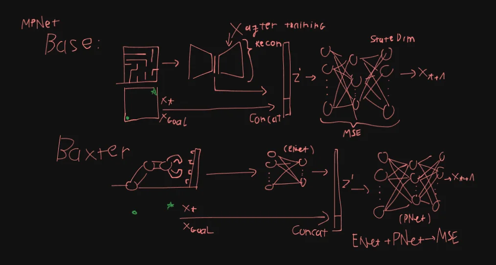
MPNet is essentially: 1 contrative autoencoders (ENet) feeding into a dense deep neural network (PNet). They train these 2 nets separately by generating synthetic workspaces, ENet is trained with reconstruction loss, while PNet is trained with MSE loss.
For the Baxter robot case, interestingly they trained the entire ENet -> PNet end-to-end with MSE loss and a shallower PNet. For ENet, they also ditched the Decoder, its a 4 layers DNN, kinda weird seeing a 4L DNN feeding into a 9L DNN but oh well.
It did worked out well for them, they state MPNet’s computation time is at least 20x faster against traditional Sampling-based Motion Planners (SMP).
My personal take is that, this paper feels kinda shaky. It feels like they run into some sort of roadblock with the Baxter robot setup (lets refer to this as Baxter MPNet) and the deadline was closing up or something.
They don’t really make justification for changing the architecture and training strategy, and their results showcase for the Baxter case is just a few lines at the end of the results section instead of a more thorough A/B/n test like they did with their base MPNet.
Another thing I found intriguing is their novel bidirectional stochastic algorithm as a heuristic for MPNet. The authors state this make the path generation heuristic “greedy and fast”.
2. Problem Definition
Let $X \subset \mathbb{R}^d$ be a given state space, $d \in \mathbb{N}$ would be 2 in $\mathbb{R}^2$ (2D space) and 3 in $\mathbb{R}^3$ (3D space).
The obstacle and obstacle-free state spaces are defined as $X_{\text{obs}} \subset X$ and $X_{\text{free}} = X\setminus X_{\text{obs}}$, respectively.
- Init state: $x_{\text{init}} \in X_{\text{free}}$
- Goal region: $X_{\text{goal}} \subset X_{\text{free}}$
- Solution path: $\tau = {x_0,x_1,\ldots,x_T}$ where $x_T \in X_{\text{goal}}$ and $x_i \in X_{\text{free}} : i = [0, T-1 ]$
3. Model Architecture
General structure: ENet and PNet.
Two phases: (A) offline training and (B) online path generation.
3.1. Base MPNet
ENet is a Contrative Autoencoder (CAE), where $\theta^e, \theta^d$ are the parameters of the encoder and decoder, respectively.
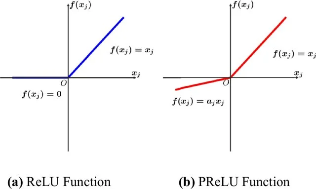
The encoding function $\text{ENet}(x_{\text{obs}})$ have 3 linear layers and 1 output layer, each linear layer is followed by the Parametric Rectified Linear Unit ($PReLU$). Input dim is a vector of point clouds of size $N_{\text{pc}} \times d_{w}$ where $N_{\text{pc}}$ is the number of data points and $d_{w} \in \mathbb{N}$ is the dimension of a workspace. Output of the encoder is $Z \in \mathbb{R}^m$ where $m \in \mathbb{N}$ is a user chosen parameter.
The decoder is simply the inverse of the encoder.
ENet is trained with reconstruction loss:
Block
Where $\lambda$ is a penalizing coefficient of user’s choosing.
After training ENet, the decoder is stripped away leaving only the encoder responsible for embedding the obstacles point cloud into $Z$.
ENet is frozen after training, then we train PNet separately, its a feed-forward deep neural network (DNN), parameterized by $\theta$ (12 layers).
Each linear layer is followed by the Parametric Rectified Linear Unit ($PReLU$). For all hidden layers in PNet, Dropout is applied with probability of $p= 0.5$. Dropout is always active despite of training or inference.
Given $Z’=\text{concat}(Z, x_{t}, x_{T})$, PNet predicts . PNet is trained with MSE loss against the human expert / classic planner feasible, near-optimal paths $\tau^*$:
Block
3.2. Baxter MPNet
For Baxter MPNet, ENet is just an encoder, in this case, its just a DNN, so we essentially have 2 DNN in this MPNet.
What’s more, PNet in Baxter MPNet is also shallower than Base MPNet with 9 layers instead of 12.
They trained Baxter MPNet end-to-end with MSE loss.
Other than that, everything else is relatively similar to Base MPNet, still $PReLU$ activation, same Dropout, same concatenation wtih $Z’$, …
4. Online Path Generation Algorithm
The online phase of MPNet performs motion planning by combining two learned components:
-
Enetencodes the obstacle point cloud into a latent obstacle representation. -
Pnetincrementally predicts intermediate states between a start and goal configuration. (autoregressive-like)
The planner operates in three stages:
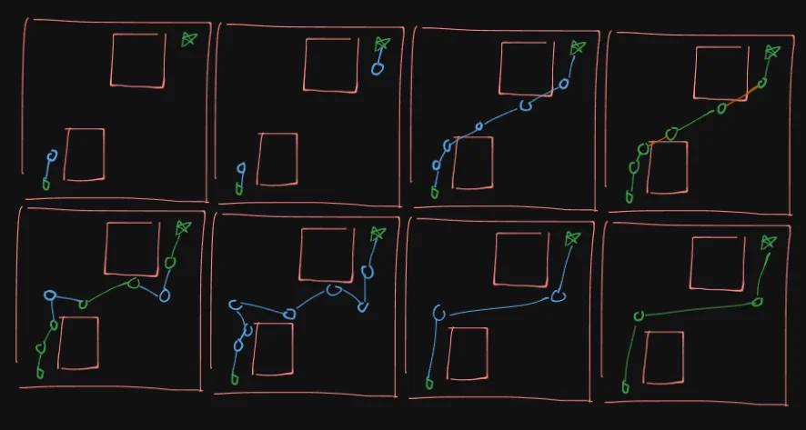
- Generate a coarse path using a bidirectional neural expansion strategy.
- Simplify the path through lazy contraction.
- Repair invalid path segments using recursive replanning.
The overall procedure is outlined below.
4.1. Overall Planning Pipeline
function MPNet(x_start, x_goal, x_obs):

    # Encode obstacle space
    z = Enet(x_obs)

    # Generate coarse path
    path = NeuralPlanner(x_start, x_goal, z)

    if path is None:
        return Failure

    # Simplify path
    path = LazyStateContraction(path)

    # Validate full trajectory
    if IsFeasible(path):
        return path

    # Repair invalid segments
    repaired_path = Replan(path, z)

    if repaired_path is None:
        return Failure

    repaired_path = LazyStateContraction(repaired_path)

    if IsFeasible(repaired_path):
        return repaired_path

    return Failure
4.2. Obstacle Encoding
The encoder network transforms the obstacle point cloud into a compact latent representation used throughout planning.
z = Enet(x_obs)
Where:
-
x_obsis the obstacle point cloud -
zis the latent obstacle embedding
This embedding remains fixed during the online planning phase.
4.3. Bidirectional Neural Path Generation
The neural planner incrementally expands two trajectories, one from the start state, one from the goal state.
At each iteration, one side predicts a new state using Pnet, then attempts to directly connect to the opposite frontier.
function NeuralPlanner(x_start, x_goal, z):

    path_a = [x_start]
    path_b = [x_goal]

    for iteration in range(max_iterations):

        # Predict next state
        x_new = Pnet(z, path_a[-1], path_b[-1])

        path_a.append(x_new)

        # Attempt direct connection
        if SteerTo(path_a[-1], path_b[-1]):

            return Concatenate(path_a, path_b)

        # Alternate expansion direction
        Swap(path_a, path_b)

    return Failure
4.3.1. Steering Function
The steering procedure checks whether two states can be connected through a collision-free linear interpolation.
function SteerTo(x1, x2):

    for δ in [0, 1]:

        x = (1 - δ) * x1 + δ * x2

        if InCollision(x):
            return False

    return True
4.3.2. Lazy State Contraction
The generated neural path may contain unnecessary intermediate states. Lazy state contraction removes redundant states by attempting direct shortcuts.
function LazyStateContraction(path):

    contracted = [path[0]]

    i = 0

    while i < len(path) - 1:

        j = len(path) - 1

        while j > i + 1:

            if SteerTo(path[i], path[j]):
                break

            j -= 1

        contracted.append(path[j])

        i = j

    return contracted
This procedure essentially acts like a lightweight path smoothing stage.
4.3.3. Path Feasibility Checking
A path is considered feasible if all consecutive state pairs are collision-free.
function IsFeasible(path):

    for i in range(len(path) - 1):

        if not SteerTo(path[i], path[i + 1]):
            return False

    return True
4.4. Recursive Replanning
If the coarse path contains invalid segments, replanning is applied locally between non-connectable states.
function Replan(path, z):

    repaired = []

    for i in range(len(path) - 1):

        x_a = path[i]
        x_b = path[i + 1]

        # Segment already valid
        if SteerTo(x_a, x_b):

            repaired.append((x_a, x_b))
            continue

        # Generate local repair path
        local_path = LocalReplanner(x_a, x_b, z)

        if local_path is None:
            return Failure

        repaired.extend(local_path)

    return repaired
The replanner can operate in two modes:
- Neural replanning: Recursively applies the neural planner on invalid local segments.
- Hybrid replanning: Falls back to a classical planner such as RRT* when neural replanning fails.
4.4.1. Neural Replanning
Neural replanning recursively refines invalid path segments.
function NeuralReplanner(x_start, x_goal, z, depth):

    if depth > max_depth:
        return Failure

    path = NeuralPlanner(x_start, x_goal, z)

    if path is None:
        return Failure

    if IsFeasible(path):
        return path

    return Replan(path, z)
4.4.2. Hybrid Replanning
Hybrid replanning integrates classical motion planning into the repair stage.
function HybridReplanner(x_start, x_goal, z):

    path = NeuralReplanner(x_start, x_goal, z)

    if path is feasible:
        return path

    # Fallback to classical planner
    return RRTStar(x_start, x_goal)
4.5. Discussion
4.5.1. Stochasticity Through Dropout
Dropout is applied during both training and inference.
x_next = Pnet(z, x_current, x_goal)
During execution, random hidden units are disabled, causing the planner to behave stochastically rather than deterministically. Consequently, repeated planning attempts can generate different trajectories for the same start and goal states. This is particularly useful during recursive replanning, where alternative paths may recover from previous failures.
4.5.2. Completeness
The neural planner alone does not provide completeness guarantees. Completeness instead depends on the replanning strategy. Pure neural replanning remains heuristic, while hybrid replanning inherits the probabilistic completeness of the underlying classical planner, such as RRT*.
4.5.3. Computational Complexity
The neural components operate with approximately constant-time inference complexity.
Enet              : O(1)
Pnet              : O(1)
Neural planning   : O(1)
Neural replanning : O(1)
(Neural networks are considered $O(1)$)
If hybrid replanning invokes a classical planner such as RRT*, the worst-case complexity becomes:
RRT* replanning : O(n log n)
In practice, they find that classical replanning is only applied to small invalid path segments rather than the full trajectory.
5. Experiments & Results
5.1. Experimental Setup
The authors implemented the proposed framework in PyTorch, while the benchmark planners, Informed-RRT* and BIT, were evaluated using Python and OMPL implementations. For the Baxter experiments, they integrated the system with ROS and MoveIt!, and compared their method against the C++ implementation of BIT. Their experiments were conducted on a machine equipped with an Intel Core i7 CPU, 32GB RAM, and an NVIDIA GTX 1080 GPU.
Their evaluation focuses on comparing MPNet with Neural Replanning (MPNet: NR) and Hybrid Replanning (MPNet: HR) against classical sampling-based planners across both low-dimensional and high-dimensional planning tasks.
5.2. Base Case(s)
5.2.1. Dataset Generation
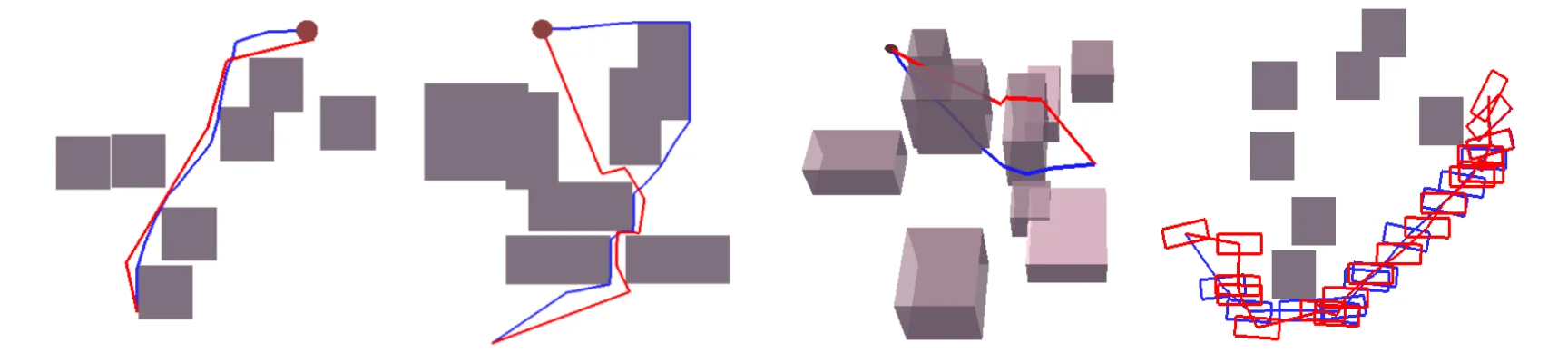
The authors evaluated their method across four planning environments: simple 2D (s2D), complex 2D (c2D), complex 3D (c3D), and rigid-body planning.
For each environment category, they generated 110 workspaces. Within every workspace, they collected 5000 collision-free near-optimal trajectories using RRT*. Their training dataset consisted of 100 workspaces with 4000 trajectories per workspace.
They constructed two separate evaluation datasets. The first, referred to as $X_\text{obs:seen}$, reused previously observed workspaces while introducing unseen start and goal configurations. The second, $X_\text{obs:unseen}$, consisted entirely of unseen workspaces and unseen planning queries.
5.2.2. Quantitative Results
The authors compared the computational time of MPNet: NR and MPNet: HR against Informed-RRT* and BIT*. Their reported metric corresponds to the time required to compute an initial feasible trajectory.
| Environment | Test Case | MPNet (NR) | MPNet (HR) | Informed-RRT* | BIT* | BIT* : t_mean / MPNet(NR) : t_mean |
|---|---|---|---|---|---|---|
| Simple 2D | Seen Xobs | 0.11 ± 0.037 | 0.19 ± 0.14 | 5.36 ± 0.34 | 2.71 ± 1.72 | 24.64 |
| Simple 2D | Unseen Xobs | 0.11 ± 0.038 | 0.34 ± 0.21 | 5.39 ± 0.18 | 2.63 ± 0.75 | 23.91 |
| Complex 2D | Seen Xobs | 0.17 ± 0.058 | 0.61 ± 0.35 | 6.18 ± 1.63 | 3.77 ± 1.62 | 22.17 |
| Complex 2D | Unseen Xobs | 0.18 ± 0.27 | 0.68 ± 0.41 | 6.31 ± 0.85 | 4.12 ± 1.99 | 22.89 |
| Complex 3D | Seen Xobs | 0.48 ± 0.10 | 0.34 ± 0.14 | 14.92 ± 5.39 | 8.57 ± 4.65 | 17.85 |
| Complex 3D | Unseen Xobs | 0.44 ± 0.107 | 0.55 ± 0.22 | 15.54 ± 2.25 | 8.86 ± 3.83 | 20.14 |
| Rigid | Seen Xobs | 0.32 ± 0.28 | 1.92 ± 1.30 | 30.25 ± 27.59 | 11.10 ± 5.59 | 34.69 |
| Rigid | Unseen Xobs | 0.33 ± 0.13 | 1.98 ± 1.85 | 30.38 ± 12.34 | 11.91 ± 5.34 | 36.09 |
Across all environment categories, their method maintained relatively stable inference time, typically remaining near one second regardless of planning dimensionality. In contrast, the execution time of Informed-RRT* and BIT* increased as the environments became more complex, particularly in rigid-body planning tasks.
They also observed that MPNet generalized beyond the environments used during training. Similar execution behavior was reported on both the $X_\text{obs:seen}$ and $X_\text{obs:unseen}$ datasets, suggesting that their learned planner retained performance in previously unseen obstacle configurations.
They however do not imply generalization across modality, for example, training in 2D and generalizing to 3D.
Examples of trajectories generated by MPNet and RRT* are shown below.
5.3. Baxter Case
5.3.1. Dataset Generation
For the Baxter experiments, the authors created ten simulated manipulation environments. In each environment, they collected 900 trajectories for training and 100 trajectories for testing.
They obtained obstacle point clouds using a Kinect depth camera together with PCL and ROS integration. Their planning task focused on generating collision-free trajectories for the 7-DOF Baxter manipulator between target joint configurations.
5.3.2. Quantitative Results
In the Baxter experiments, the authors compared MPNet against BIT* in a high-dimensional manipulation setting. Their method achieved approximately one-second planning time on average while maintaining a relatively high success rate across the test environments. BIT*, although capable of generating feasible trajectories, required substantially longer execution time, particularly when constrained to path quality comparable to MPNet.
Their results suggest that the neural planner remained computationally stable even in high-dimensional manipulation tasks, whereas the execution time of classical sampling-based planning varied more significantly.
6. Final Thoughts
I’m gonna put my full thoughts in the Motion Planning Transformers post here (coming soon). I already have some quick personal notes in 1. Recap.