Text-to-SQL SLM: Finetuning Gemma 3 with QLoRA
Access Links
- 👨💻 Model & Code: Yuk050/gemma-3-1b-text-to-sql-model
- 🤗 HuggingFace Space: Yuk050/gemma-3-1b-text-to-sql
- ⌛ The project spanned from June 26th, 2025 till around the end of June.
Prologue
Honestly, I don’t really see much value in doing a project like this one. In my opinion, as of now working with LLMs, especially in research, is still quite informal and chaotic, I probably will make a separate post to talk about this more in depth, but basically, I believe that, unless given the clear cut goal, rigorous backing, and most importantly compute, then “LLM research” is still quite insignificant to me. Nevertheless, because of my recent aspirations, and the fact that, I do want to try everything before having a say about them, leads to this project. Yeah, this is probably the most “project for the sake of projects” among my list as of now, but you know what, better than doing nothing I guess, and I can say I tried it at least, not gonna have a lot to say about this one though, probably just gonna cover the math which is somewhat intriguing.
Table of Content
Block
Project Overview
Only meaningful math here is QLoRA I guess, other stuff, I will cover briefly, some refresher can’t hurt. The project is exactly what it sounds like:
- A Text-to-SQL Dataset: Synthetic Text-to-SQL (gretelai/synthetic_text_to_sql)
- An SLM (Small Language Model): Gemma 3 1B (google/gemma-3-1b-it)
- Finetuning method: QLoRA (Dettmers et al., 2023)
- Hugging Face deployment: Spaces (Hugging Face Spaces)
Pretty straightforward: Finetune a Gemma 3 1B model for the text-to-SQL task using QLoRA, deploy on Hugging Face Spaces. With these primers to finetuning, I recommend Unsloth, they provide a ton of resources on working with LLMs and my notebook is even heavily based on their collection of starter notebooks. You can literally just load up one of their pre-made notebooks in Google Colab, dive in and try stuff, with those-being able to say that you “did finetuning” is kinda trivially easy.
But yeah, that alone did not satisfy me, so i delved into the math of QLoRA, and its quite interesting, more interesting than most LLM research I suppose.
Text-to-SQL Task
Not much to say here, I guess one of the best way to get familiar with this concept is to go to any Data Studio page of a dataset hosted on Hugging Face, for example: gretelai/synthetic_text_to_sql/viewer. To the right you will immediately see a section with a chatbox that prompts “Ask AI to help write your query…“. This is what I consider to be the gold standard in terms of handling a text-to-SQL task.
In its simplest form, you are going to need: full schema-context of an SQL table + a natural language query to be able to perform this task meaningfully, as going from just a natural language query to SQL query without any schema is ill-posed and honestly kinda shady. But I have seen models that do just that on Hugging Face before, so yeah watch out for that, you NEED schemas.
Lets take an sample from our dataset to examine a real example, suppose we have this SQL table:
| id | cost | type |
|---|---|---|
| 1 | 500 | Insulation |
| 2 | 1000 | HVAC |
| 3 | 1500 | Lighting |
That were created with this SQL schema context:
CREATE TABLE upgrades (
    id INT,
    cost FLOAT,
    type TEXT
);

INSERT INTO upgrades (id, cost, type) VALUES
    (1, 500, 'Insulation'),
    (2, 1000, 'HVAC'),
    (3, 1500, 'Lighting');
If just given this natural language question: “Find the energy efficiency upgrades with the highest cost and their types.”, a model might output something like:
SELECT
    u.cost,
    ut.type_name
FROM
    upgrades AS u
JOIN
    upgrade_types AS ut ON u.upgrade_type_id = ut.type_id
WHERE
    u.cost = (SELECT MAX(cost) FROM upgrades);
Running the actual SQL query gives:
Error: no such table: upgrade_types
But if you include the SQL schema context into the prompt, the model responses with:
SELECT
    cost,
    type
FROM
    upgrades
WHERE
    cost = (SELECT MAX(cost) FROM upgrades);
Running this query outputs:
| cost | type |
|---|---|
| 1500 | Lightning |
Meanwhile the groundtruth SQL query from the dataset for this sample is:
SELECT
    type,
    cost
FROM
    (SELECT
        type,
        cost,
        ROW_NUMBER() OVER (ORDER BY cost DESC) AS rn
    FROM
        upgrades
    ) AS sub
WHERE
    rn = 1;
And running the groundtruth query gives:
| cost | type |
|---|---|
| 1500 | Lightning |
So 2 things to take note of:
- You need schema, if its not present then the SQL query is wishful thinking.
- Best way to evaluate performance is to run the actual SQL query in a console (I used Programiz Online SQL Compiler for quick checking)
Having rarely touched SQL queries before, this feature on Hugging Face was a huge help for my projects, I mean sooner or latter im gonna have to pick up some SQL anyway, but its one of those thing that I think is not really about any sort of “learning” in terms of coding, rather its mostly just syntax memorization.
Nevertheless, this task have broad implications, whether it be in apps like that Hugging Face feature, for propriety use in a company for employees, and so on.
Gemma 3
Gemma 3 is a recent State-of-the-art (SOTA) open-source family of models from Google. You can checkout this model from a plethora of sources already. I picked this model mostly because I expect to be working with them more in the future, they are quite decent.
In this project, I chose the 1 billion parameter google/gemma-3-1b-it, there was already plenty of resources on finetuining this particular model.
QLoRA
This is where the bulk of the math is, and probably the only part that I had fun with during this project lmao. So, QLoRA (LoRA stands for Low-rank Adaptation, Q here most likely mean Quantization-aware), to really get to its roots I recommend reading these papers in order:
- Frantar et al., 2023: Roots of quantizing LLMs, different quantization methods for LLMs.
- Hu et al., 2021: Original LoRA paper, fundamental concepts are here, QLoRA builds upon LoRA by considering quantized models
- Dettmers et al., 2023: The QLoRA paper.
Also, I highly recommend these videos for QLoRA:
So, lets go over a few primers:
Quantization for LLMs
Quantization, in the context of Large Language Models (LLMs), is a technique that reduces the precision of the numerical representations of a model’s weights and activations. Instead of using high-precision floating-point numbers (like FP32), quantization converts them to lower-precision formats (like INT8 or INT4). This process offers significant benefits, primarily in reducing memory footprint and accelerating inference speed, making LLMs more accessible on resource-constrained hardware, such as consumer-grade GPUs or edge devices.
At its core, quantization is about trading off a small amount of precision for substantial gains in efficiency. The fundamental concept is to map a range of floating-point values to a smaller set of integer values. This mapping involves a scale factor and often a zero-point (offset) to ensure that the quantized values accurately represent the original range. The formula for uniform quantization is typically q = round(r / S) + Z, where q is the quantized integer, r is the real-valued floating-point number, S is the scale factor, and Z is the zero-point. The inverse operation, dequantization, recovers an approximation of the original floating-point value: r_approx = (q - Z) * S.
Why Quantization?
The primary motivations behind quantizing LLMs are clear: memory and speed. Modern LLMs can have billions or even trillions of parameters, each typically stored as a 32-bit floating-point number. This leads to massive model sizes (e.g., a 7B parameter model requires approximately 28 GB of memory in FP32 precision). Such large memory requirements make it challenging to load and run these models on consumer hardware. By reducing the precision to, say, 4-bit integers, the memory footprint can be reduced by 8x, making it feasible to run larger models on smaller GPUs. This memory reduction also translates directly into faster inference times, as less data needs to be moved between memory and processing units.
Static vs. Dynamic Quantization
Quantization methods can be broadly categorized into static and dynamic, based on when the quantization parameters (scale and zero-point) are determined:
- Dynamic Quantization: In dynamic quantization, weights are quantized offline (statically), but activations are quantized on-the-fly during inference. This means the scale and zero-point for activations are computed dynamically for each input tensor. This approach is simpler to implement and generally offers better accuracy than static quantization for activations, as it adapts to the actual range of values during runtime. However, the overhead of computing these parameters at runtime can introduce latency, making it less ideal for latency-sensitive applications.
- Static Quantization (Post-Training Static Quantization - PTSQ): Static quantization determines the quantization parameters for both weights and activations before inference, typically by running a calibration dataset through the model. This pre-computation eliminates the runtime overhead of dynamic quantization, leading to faster inference. However, it requires a representative calibration dataset, and the fixed quantization ranges might not perfectly capture the full range of values during actual inference, potentially leading to a slight drop in accuracy compared to dynamic quantization or full-precision models. For LLMs, static quantization is often preferred for maximizing throughput and reducing latency due to their computational intensity.
Uniform vs. Non-Uniform Quantization
Another distinction in quantization schemes is whether the quantization intervals are uniform or non-uniform:
- Uniform Quantization: This is the simplest form, where the value range is divided into equally spaced intervals. Each interval is mapped to a unique integer. While straightforward to implement, uniform quantization can be suboptimal for data distributions that are not uniform, such as the weight distributions in neural networks, which often follow a bell-shaped curve (e.g., Gaussian). Outliers in the distribution can disproportionately affect the quantization range, leading to reduced precision for the majority of values.
- Non-Uniform Quantization: This approach uses non-uniform spacing for the quantization intervals, allowing for finer granularity in regions where the data is more concentrated (e.g., around zero for weight distributions) and coarser granularity for less frequent values (outliers). This can lead to higher accuracy for a given bit-width compared to uniform quantization, as it better captures the underlying data distribution. NormalFloat 4 (NF4), used in QLoRA, is a prime example of a non-uniform quantization scheme.
Bit-level Layout of Q4 (and the Q_K/M/S Terminology)
When you encounter terms like Q4_K, Q4_M, or Q4_S in the context of quantized LLMs, especially with ggml or GGUF formats, it refers to specific 4-bit quantization schemes that optimize for different trade-offs between model size, performance, and accuracy. The K in Q_K often refers to k-quant methods, which are generally designed to have less perplexity loss relative to their size .
Let’s demystify the Q_4_K/M/S terminology and connect it with practical implications. The Q signifies quantization, and 4 indicates 4-bit precision. The suffixes (K, M, S) denote variations in how the 4-bit quantization is applied, particularly concerning block sizes and the handling of scaling factors and zero-points.
In essence, 4-bit quantization means that each original 32-bit floating-point value is compressed into a 4-bit integer. A 4-bit integer can represent 2^4 = 16 distinct values. For example, if we have a range of [-1.0, 1.0] and we uniformly quantize it to 4 bits, each step would be 2.0 / 15 (since there are 15 intervals between 16 values). The original floating-point value is then scaled and rounded to fit into one of these 16 integer bins.
However, simple uniform 4-bit quantization can lead to significant accuracy loss, especially for LLMs. This is where the more advanced Q_K variants come in. These methods often employ a block-wise quantization strategy, where weights are grouped into blocks, and each block has its own scaling factor and zero-point. This allows for more granular control over the quantization process, adapting to local variations in weight distributions.
-
Q4_K: This is a family of 4-bit quantization methods that often involve hybrid quantization, where some parts of the model (e.g., important layers or outliers) might be quantized to a higher precision (e.g., 5-bit or 6-bit) while the majority remains at 4-bit. This aims to preserve critical information while still achieving significant compression.
Q4_Kmodels generally offer a good balance between size and performance. -
Q4_K_M: The
Moften stands forMedium, suggesting a balance between size and quality. These models are often recommended for general use as they provide a good compromise between perplexity (a measure of how well a probability distribution predicts a sample) and model size. I often find myself usingQ4_K_Mfor my own experiments when I’m not usingQ8_0. -
Q4_K_S: The
Stypically stands forSmall, indicating a model that is more aggressively compressed, resulting in a smaller file size but potentially lower quality (higher perplexity) compared toQ4_K_M. These models are suitable for scenarios where memory or storage is extremely limited.
Here’s a simplified table to compare these quantization schemes:
| Quantization Scheme | Description | Use Case |
|---|---|---|
| Q8_0 | 8-bit quantization. Offers the best quality among quantized models, with a larger file size. | When you want the best possible performance from a quantized model and have sufficient VRAM. |
| Q4_K_M | 4-bit quantization with a medium level of compression. A good balance between model size and performance. | General use, especially on consumer GPUs where VRAM is a constraint. |
| Q4_K_S | 4-bit quantization with a high level of compression. The smallest file size, but with a potential trade-off in performance. | When memory or storage is extremely limited, and you’re willing to sacrifice some performance. |
| NF4 | 4-bit NormalFloat. A non-uniform quantization scheme that is information-theoretically optimal for normally distributed data (like LLM weights). | Used in QLoRA for fine-tuning, as it preserves more information than uniform 4-bit quantization. |
At first, I was also confused with all the tags like Q_8, Q_4, etc., when working with open-source LLMs. My personal preference is to use Q8_0 for the best quality, but Q4_K_M is perfectly fine for experimentation and when VRAM is a concern.
Intuition of LoRA
Now, let’s get to the heart of the matter: LoRA, or Low-Rank Adaptation. The core idea behind LoRA is to make the fine-tuning of large language models more efficient by drastically reducing the number of trainable parameters. Full fine-tuning, where you update all the weights of a massive model, is incredibly expensive, both in terms of computational resources and memory. LoRA provides a clever workaround.
Instead of updating the entire weight matrix W of a pre-trained model, LoRA freezes W and injects a pair of smaller, trainable matrices, A and B, into each layer of the model. The update to the weight matrix, ΔW, is then represented by the product of these two smaller matrices: ΔW = A * B. This is where the “low-rank” part comes in. The rank of a matrix is a measure of its complexity, and by decomposing the weight update into two smaller matrices, we are essentially approximating the full-rank update with a low-rank one.
Let’s look at the dimensions to understand the parameter reduction. If the original weight matrix W has dimensions d x k, then the update ΔW also has dimensions d x k. In LoRA, the matrix A has dimensions d x r and B has dimensions r x k, where r is the rank and is much smaller than d and k (r << min(d, k)). The number of trainable parameters in LoRA is r * d + r * k = r * (d + k), whereas the number of parameters in the original weight matrix is d * k. Since r is small, r * (d + k) is significantly smaller than d * k, leading to a massive reduction in the number of trainable parameters.
For example, if we have a layer with d = 4096 and k = 4096, and we choose a rank r = 8, the number of trainable parameters in LoRA would be 8 * (4096 + 4096) = 65,536. In contrast, the original weight matrix has 4096 * 4096 = 16,777,216 parameters. That’s a reduction of over 250x in the number of trainable parameters for that layer!
This low-rank approximation works because the updates to the weights during fine-tuning have been shown to have a low intrinsic rank. In other words, the changes needed to adapt a pre-trained model to a new task are often low-dimensional, and LoRA cleverly exploits this property.
Here’s a diagram illustrating the difference between a standard fine-tuning update and a LoRA update:
Standard Fine-Tuning:
   +-----------------+     +-----------------+     +-----------------+
   |   Input (x)     | --> |   Pre-trained   | --> |   Output (h)    |
   |                 |     |   Weight (W)    |     |                 |
   +-----------------+     +-----------------+     +-----------------+
                                   |
                                   v
                              +---------+
                              |  ΔW     |
                              +---------+
LoRA Fine-Tuning:
   +-----------------+     +-----------------+     +-----------------+
   |   Input (x)     | --> |   Pre-trained   | --> |   Output (h)    |
   |                 |     |   Weight (W)    |     |                 |
   +-----------------+     +-----------------+     +-----------------+
                                   |
                                   v
                              +---------+     +---------+
                              |    A    | --> |    B    | --> ΔW
                              +---------+     +---------+
Math of QLoRA
QLoRA takes the efficiency of LoRA a step further by combining it with quantization. It allows for fine-tuning quantized models, which was previously not possible without significant performance degradation. QLoRA introduces three key innovations: 4-bit NormalFloat (NF4), double quantization, and paged optimizers.
NormalFloat 4 (NF4)
As we discussed earlier, NF4 is a non-uniform 4-bit quantization scheme that is information-theoretically optimal for normally distributed data. This is crucial because the weights of pre-trained neural networks are typically normally distributed. Unlike uniform quantization, which uses evenly spaced quantization levels, NF4 uses quantiles to create the quantization bins. This means that the bins are more densely packed around the center of the distribution (where most of the weights are) and more spread out in the tails. This allows NF4 to represent the original weight distribution with higher fidelity than uniform 4-bit quantization, leading to better performance.
To be more specific, NF4 is a data type that has an equal number of expected values in each quantization bin. It is built upon Quantile Quantization, which is a method that ensures each quantization bin has the same number of values from a source distribution. This is achieved by estimating the quantiles of the source distribution and then assigning the mean of the values in each bin as the representative value for that bin. This process results in a non-uniform quantization scheme that is highly effective for normally distributed data.
Let’s try to manually map some real numbers to NF4. Suppose we have the following numbers: [0.01, -0.25, 0.6, -1.2]. The first step would be to normalize these values to a standard normal distribution. Then, we would use the pre-computed quantiles of the standard normal distribution to determine the appropriate 4-bit integer representation for each value. The exact mapping would depend on the specific NF4 implementation, but the key idea is to use the quantiles to create a non-uniform mapping that preserves the most important information in the data.
Double Quantization
Double quantization is a clever trick to further reduce the memory footprint of the quantization process. When we quantize a model, we need to store the quantization parameters (scale and zero-point) for each block of weights. These parameters are typically stored in a higher-precision format (e.g., FP32), which can add up to a significant amount of memory overhead. Double quantization addresses this by quantizing the quantization constants themselves.
In essence, we perform a second level of quantization on the scaling factors. This is done by grouping the scaling factors into blocks and then quantizing them using a lower-precision format (e.g., 8-bit). This reduces the memory required to store the quantization metadata, leading to further memory savings. The authors of the QLoRA paper found that this technique can save up to 0.5 bits per parameter on average, which is a significant reduction when dealing with billions of parameters.
Paged Optimizers
Finally, QLoRA introduces paged optimizers to handle memory spikes during training. When we fine-tune a model, the optimizer (e.g., AdamW) needs to store the optimizer states (e.g., momentum and variance) for each trainable parameter. For large models, these optimizer states can consume a significant amount of GPU memory. Paged optimizers use a feature of NVIDIA GPUs called unified memory to automatically page the optimizer states between the GPU and CPU memory. This means that when the GPU runs out of memory, the optimizer states are automatically moved to the CPU RAM, and then moved back to the GPU when they are needed. This allows us to fine-tune much larger models on a single GPU than would otherwise be possible.
QLoRA in Practice
So, how does all of this come together in practice? The workflow for using QLoRA is surprisingly simple, thanks to libraries like bitsandbytes and peft (Parameter-Efficient Fine-Tuning) from Hugging Face, and of course, Unsloth, which makes it even easier.
Here’s a high-level overview of the steps involved:
-
Load the model in 4-bit: The first step is to load the pre-trained model in 4-bit precision. This is typically done by setting the
load_in_4bit=Trueflag when loading the model using thefrom_pretrainedmethod from thetransformerslibrary. You’ll also specify the 4-bit quantization type, such asnf4. -
Apply LoRA on top: Once the model is loaded in 4-bit, you apply LoRA on top of it using the
peftlibrary. This involves creating aLoraConfigobject where you specify the LoRA parameters, such as the rank (r), the LoRA alpha (lora_alpha), and the target modules (the layers of the model where you want to apply LoRA). -
Train only the adapters: With the LoRA adapters in place, you can now train the model. The key here is that you only train the LoRA adapters, while the original pre-trained weights remain frozen. This is what makes the training process so efficient. You’ll also use a paged optimizer, such as
paged_adamw_8bit, to manage memory usage during training. - Save only the LoRA adapters: After training is complete, you only need to save the LoRA adapters, not the entire model. This results in a very small checkpoint file (typically a few megabytes), which makes it easy to share and deploy the fine-tuned model.
Here’s a simplified code snippet to illustrate the process:
from transformers import AutoModelForCausalLM, AutoTokenizer, BitsAndBytesConfig
from peft import get_peft_model, LoraConfig

# Load the model in 4-bit
quantization_config = BitsAndBytesConfig(load_in_4bit=True, bnb_4bit_compute_dtype="bfloat16", bnb_4bit_quant_type="nf4")
model = AutoModelForCausalLM.from_pretrained("google/gemma-3-1b-it", quantization_config=quantization_config)

# Apply LoRA on top
lora_config = LoraConfig(r=8, lora_alpha=32, target_modules=["q_proj", "k_proj", "v_proj", "o_proj"], lora_dropout=0.05, bias="none", task_type="CAUSAL_LM")
model = get_peft_model(model, lora_config)

# Train the model (training code omitted for brevity)

# Save the LoRA adapters
model.save_pretrained("gemma-3-1b-it-lora-adapters")
And yeah thats about it. With just a few lines of code, you can fine-tune a massive language model on a single consumer-grade GPU, thanks to the power of QLoRA. It’s a game-changer for democratizing access to large language models and enabling a wide range of new applications.
Hugging Face Deployment
Easy place to deploy LLM and AI/ML projects? Hugging Face Spaces. Its a git-based interface so it should be familiar to all partitioners, furthermore they provide generous free hosting, hardware, and accessible UI. Perfect for this kind of project.
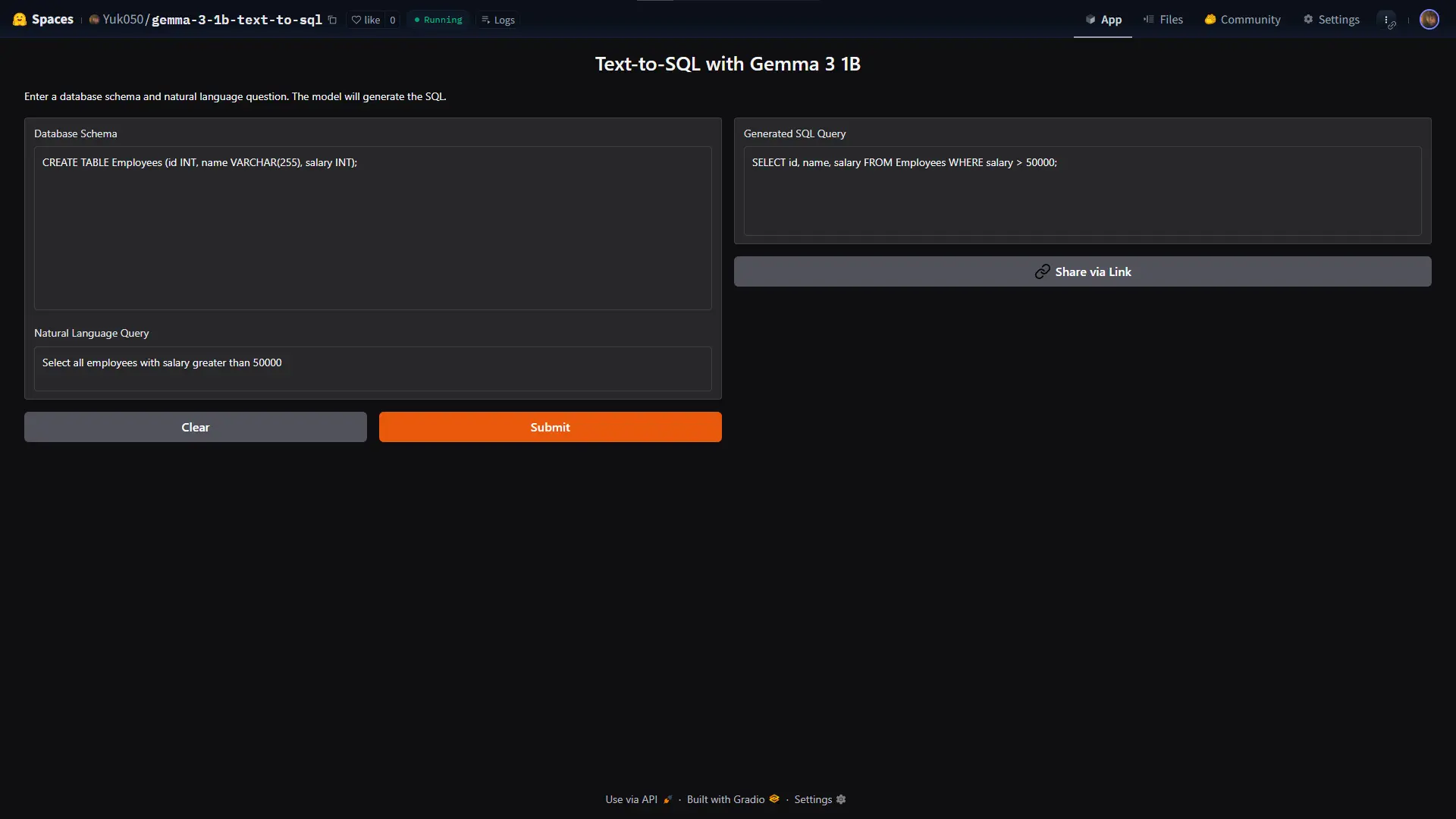
You can try the finetuned model right now by visiting Yuk050/gemma-3-1b-text-to-sql.
Epilogue
So yeah, I was mostly doing this project for the math (of which is not that relevant to the project anyway). Nevertheless, now I can say I did it, I do want to give some thoughts on the current state of LLM practices though. As of July 2025, I kinda feel like its not exactly worth it to just do these kind of projects for projects sake, as the landscape is extremely vast and non-formal. An endless flavor of LLMs (Llama, Qwen, Gemma, Aya, Jan nano, etc…) means each and everyone of them have there own little quirks, not to mention, sometimes you might even run into troubles that are hardware-specific. Weird numeric handling, different quantization format, the blackbox nature that is STILL not addressed, yeah, unless the goal post is clear and the miscellaneous is clean, i dont recommend picking up one of these projects for fun. I believe that my finetuning only worked that fast is because I based it off the Unsloth notebook.
But, I had some fun I suppose, one more step towards grasping all thing LLMs, I’m looking forward to try some RLHF (Reinforcement Learning from Human Feedback), so until then, thanks for reading.