Table of Content

• Table of Content
• Overview
• Hard Margin SVM
• Linearly Separable Data
• Margin of a Separating Hyperplane
• Constrained Optimization Problem
• Lagrangian Dual Problem
• Quadratic Programming
• Final model
• Soft Margin SVM
• Nearly Linearly Separable Data
• Approach: Quadratic Programming
• Approach: Gradient Descent
• Kernel SVM
• Non-Linear Data
• Kernel Function and Kernel Trick
• Building the Optimization Problem
• Final Model
• Extra: SVM for Multiclass Classification
• References

Block

Overview

Support Vector Machine (SVM) is a family of model that leverage the concept of Support Vector to find boundaries that best separate the data. The most basic usage for SVM is in binary classification with linearly separable or nearly linearly separable data. In such cases, SVM will find the most optimal hyperplane that best separate the two classes into a positive region and a negative region in relation to the two binary classes.

Moreover, SVM can also be used for regression and multiclass classification by extension of multiple binary SVM models. Most importantly, by utilizing kernel functions and the kernel trick, SVM is one of the few classical model that can handle non-linear data efficiently with unprecedented flexibility. However, SVM is noticeably prone to overfitting and both train and inference time can take exponentially longer as data grows. Furthermore by not relying on a statistical or similarity basis like that of Logistic Regression or K-NN, SVMs are also somewhat harder to interpret with its underlying geometric approach.

We will now discuss Hard Margin SVM for linearly separable data, Soft Margin SVM for nearly linearly separable data and Kernel SVM for non-linear data.

Hard Margin SVM

Linearly Separable Data

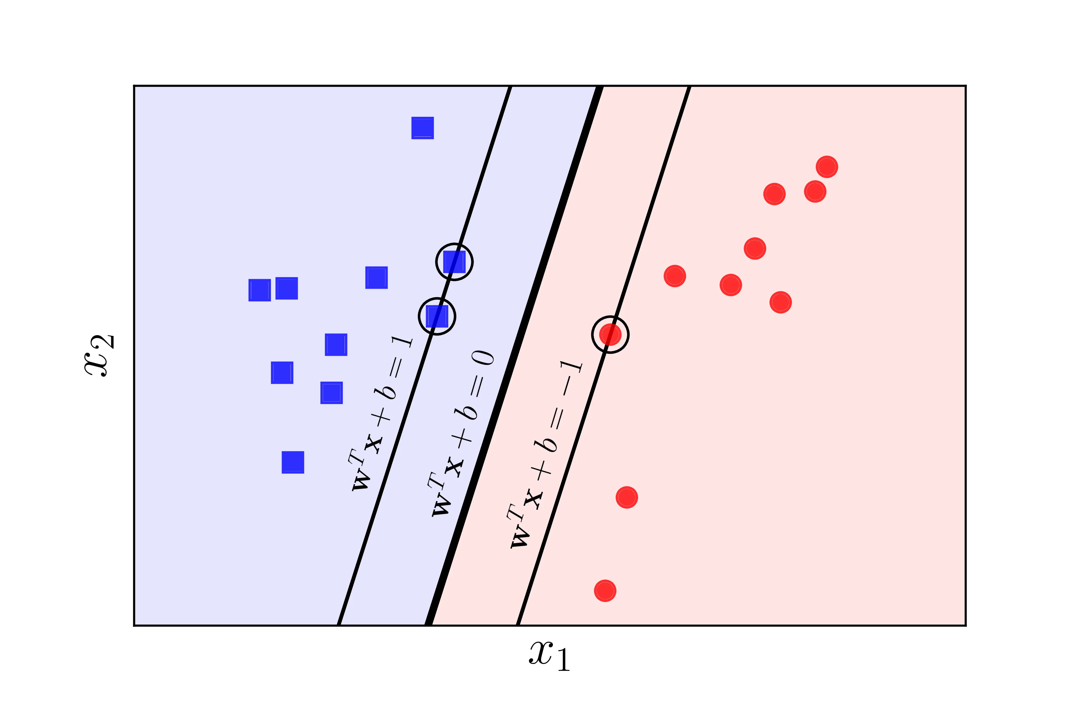
Given dataset $X = \{(\mathbf{x}_i, y_i)\}^N_{i=1}$ where $\mathbf{x}_i \in \mathbb{R}^n$ and $y_i \in \{-1, +1\}$, this is a binary classification task. Let $X$ be linearly separable, assume the SVM model has already found the optimal separating hyperplane $H_0 : \mathbf{w}^\top \mathbf{x} + b$, we can visualize with an example in $\mathbb{R}^2$ ($H_0$ is a line in this case):

Margin of a Separating Hyperplane

We define the distance from a data point $\mathbf{x}_i$ to $H_0$ as:

$$d_i = \frac{|\mathbf{w}^\top \mathbf{x}_i + b|}{\|w\|_2} \quad$$

Block

If we remove $\mid \cdot \mid$ on the numerator and in figure 1 we define the left is the positive region (blue) and the right is the negative region (red), then we will be able to know which region does $\mathbf{x}_i$ belongs to:

$$d_i = \frac{\mathbf{w}^\top \mathbf{x}_i + b}{\|w\|_2} \quad$$

Block

Let $d_+$ and $d_-$ be the minimal distance from any data point from the positive and negative region respectfully that is closest to hyperplane $H_0$. We can define the margin with width $d_+ + d_-$ (2 slim line on both side of $H_0$ in figure 1). For $H_0$ to be optimal, we must ensure that no data point is inside the margin. For that, we formulate the constraints:

$$\begin{gather} \mathbf{w}^\top \mathbf{x}_i + b \geq +1 \quad \text{for} \quad y_i = +1 \quad \\ \mathbf{w}^\top \mathbf{x}_i + b \leq -1 \quad \text{for} \quad y_i = -1 \quad \end{gather}$$

Block

The constraints above can be combined into a single constraint:

$$y_i(\mathbf{w}^\top \mathbf{x}_i + b)-1 \geq 0, \forall i \quad$$

Block

Constrained Optimization Problem

Note that $\mathbf{w}^\top \mathbf{x}_i + b = +1$ $\implies \mathbf{x}_i \in H_1 :$ $\mathbf{w}^\top \mathbf{x} + b = +1$ and $\mathbf{w}^\top \mathbf{x}_j + b = -1$ $\implies \mathbf{x}_j \in H_2 :$ $\mathbf{w}^\top \mathbf{x} + b = -1$. All such $\mathbf{x}_i, \mathbf{x}_j$ are called support vectors (circled points in figure 1). Thus, we have the width of our margin as:

$$d_+ + d_- = \frac{1}{\|\mathbf{w}\|_2} + \frac{1}{\|\mathbf{w}\|_2} = \frac{2}{\|\mathbf{w}\|_2} \quad$$

Block

The goal of hard margin SVM is to find the optimal separating hyperplane $H_0$ while also maximizing the width of the margin, thus we formulate the constrained optimization problem:

$$\min_{w, b} \frac{1}{2}\|\mathbf{w}\|_2^2 \quad \text{subject to} \quad y_i(w^\top x_i + b) \geq 1 , \forall i \quad (1) \quad$$

Block

The constraint ensure that no data point will lie inside the margin, aiding in making sure that class $+1$ and $-1$ is perfectly separated, thus “hard margin”.

Lagrangian Dual Problem

Solving $(1)$ directly is quite challenging, thus we derive the Lagrangian primal:

$$\mathcal{L}_P = \frac{1}{2}\|\mathbf{w}\|_2^2 - \sum^N_{i=1} \alpha_i \left[ y_i(\mathbf{w}^\top \mathbf{x}_i + b)-1\right] \quad (2) \quad$$

Block

Where $\boldsymbol{\alpha} = \{\alpha_1, \alpha_2, \ldots, \alpha_N\} \mid \alpha_i \geq 0, \forall i$ are the Lagrange multipliers for each data points. The most important aspect about $(2)$ is that we can derive the Lagrangian dual problem for $(1)$. Now we may check a few conditions that are crucial for the SVM model in general:

In $(1)$, $\frac{1}{2}\|\mathbf{w}\|_2^2$ is a convex function and the constraints are linear, thus $(1)$ is a convex optimization problem. Furthermore, due to $X$ being linearly separable, we know that:

$$\text{Feasible set} \neq \emptyset \implies \exists (\mathbf{w}, b) \mid y_i(\mathbf{w}^\top \mathbf{x}_i + b) > 1, \forall i \quad$$

Block

Thus the Slater condition is satisfied and strong duality occurs, ensuring that the solution to the primal $(2)$ is equivalently optimal as the solution to the dual problem:

$$\text{Primal Objective Value} = \text{Dual Objective Value} \quad$$

Block

In $(2)$ the Karush-Kuhn-Tucker conditions (KKT) is satisfied:

$$\begin{align*} \text{Primal feasibility: } & y_i(\mathbf{w}^\top \mathbf{x}_i+b)-1 \geq 0 \\ \text{Dual feasibility: } & \alpha_i \geq 0 \\ \text{Complementary slackness: } & \alpha_i \left[y_i(\mathbf{w}^\top \mathbf{x}_i+b)-1\right]=0 \quad \\ \end{align*}$$

Block

$$\begin{gather*} \text{Stationary:} \\ \text{For } \mathbf{w}: \frac{\partial\mathcal{L}_P}{\partial w_v} = w_v - \sum^N_{i=1} \alpha_i y_i \mathbf{x}_i = 0, \forall v = 1, \ldots n \quad \\ \text{For } b: \frac{\partial\mathcal{L}_P}{\partial b} = \sum^N_{i=1} \alpha_i y_i = 0 \end{gather*}$$

Block

The KKT conditions is necessary and sufficient to provide us with an solution to the dual problem that is most optimal. The complementary slackness condition built from the primal and dual feasibility ensure that only support vectors will affect the solution which aligns with the objective of SVM. The stationary conditions directly help us compute $\mathbf{w}, b, \boldsymbol{\alpha}$.

We may now construct the Lagrangian dual problem for $(2)$ using the derivatives calculated from the KKT conditions, we substitute:

$$\mathcal{L}_D = \sum^N_{i=1} \alpha_i - \frac{1}{2} \sum^N_{i=1} \sum^N_{j=1} \alpha_i \alpha_j y_i y_j \mathbf{x}_i^\top \mathbf{x}_j \quad (3) \quad$$

Block

Quadratic Programming

Let $H_{ij} = y_i y_j \mathbf{x}_i^\top \mathbf{x}_j$, we construct a new constrained optimization problem for $(3)$:

$$\max_{\boldsymbol{\alpha}} \sum^N_{i=1} \alpha_i - \frac{1}{2} \boldsymbol{\alpha}^\top \boldsymbol{H} \boldsymbol{\alpha} \quad \text{subject to:} \quad \alpha_i \geq 0, \forall i \quad ; \quad \sum^N_{i=1} \alpha_i y_i = 0 \quad (4) \quad$$

Block

We can solve $(4)$ with quadratic programming algorithms such as direct QP ($O(n^3)$), Sequential Minimal Optimization (SMO) ($O(n^2)$),…

Assume the quadratic solver provide us with the solution, meaning the optimal $\boldsymbol{\alpha}^{'} \in \mathbb{R}^N \mid \alpha_i^{'} \geq 0$. Note that because of complementary slackness of KKT, all points where $\alpha_i^{'} > 0$ will be support vectors, assume $S$ is the set of all support vectors, then most likely, $\mid S \mid << \mid X \mid$ and $\alpha_i^{'} = 0$ for all $\mathbf{x}_i \notin S$. Then, based on the stationary conditions, we may compute $\mathbf{w}$ and $b$:

$$\begin{gather*} \mathbf{w} = \sum^N_{i=1} \alpha_i^{'} y_i \mathbf{x}_i \\ b = \frac{1}{|S|} \sum_{i \in S} \left(y_i - \sum_{j \in S} \alpha_i^{'} y_j (\mathbf{x}_i^\top \mathbf{x}_j) \right) \quad \end{gather*}$$

Block

Final model

After obtaining $\mathbf{w}$ and $b$, the model will be able to make prediction for query point $\mathbf{x}_q \in \mathbb{R}^n$:

$$y_q = \text{sign}(\mathbf{w}^\top \mathbf{x}_q +b) \quad$$

Block

Soft Margin SVM

Nearly Linearly Separable Data

In reality, very rarely is data actually linearly separable like in figure 1, we may observe an example in $\mathbb{R}^2$:

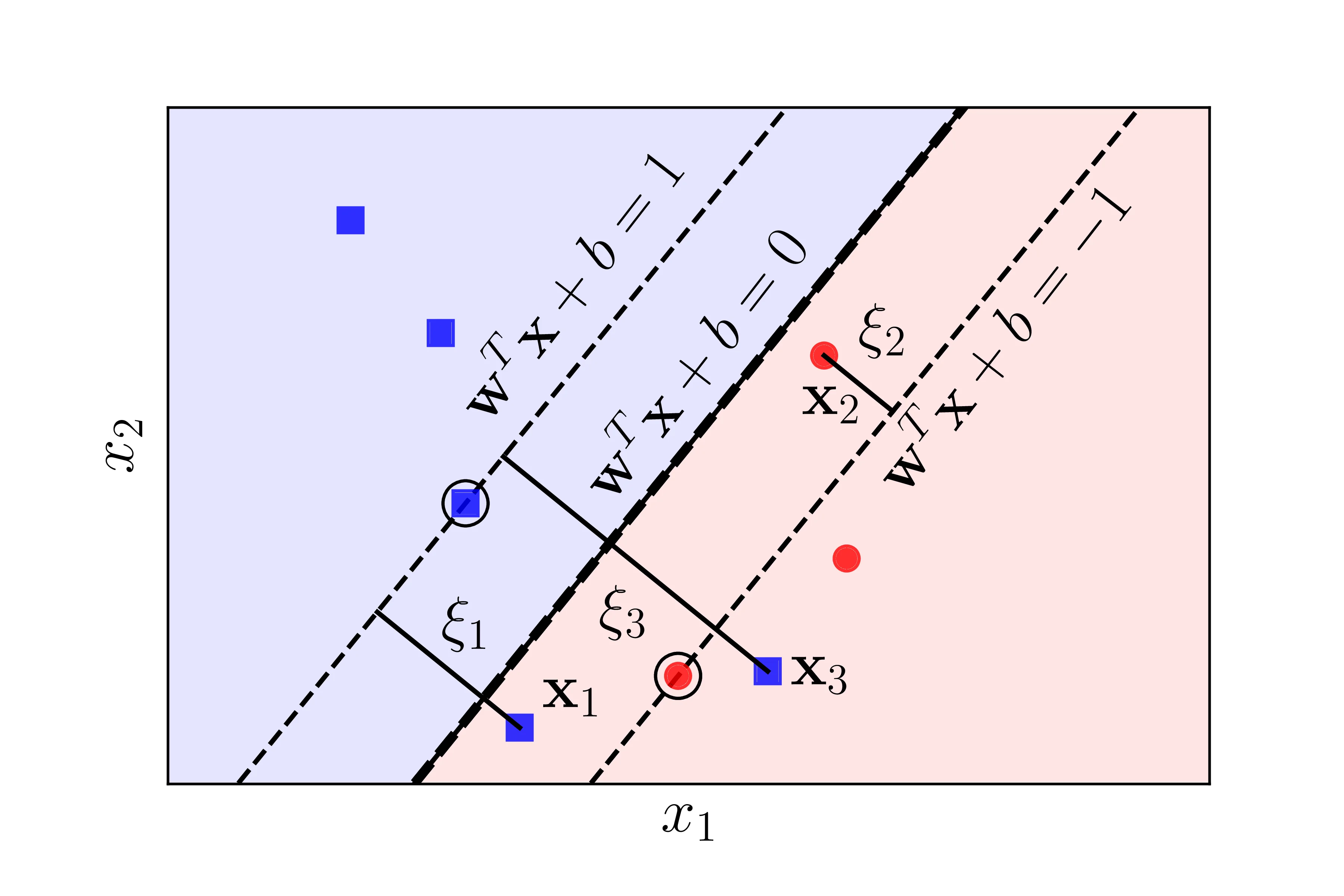
The case above is called nearly linearly separable data. For $\mathbf{x}_2$, the data point is dangerously close to $H_0$ and is inside the margin. If we follow through with our constraint that all point mustn’t lie inside the margin the we would have a very narrow margin, thus reducing generalizability. For points like $\mathbf{x}_1$ and $\mathbf{x}_3$, its even impossible to construct a hyperplane that can actually completely separate the two classes.

The aforementioned drawbacks are the fundamental limitations of hard margin SVM. By not defining the constraint to be strict, we could build the soft margin SVM model to handle nearly linearly separable data. To achieve this, we introduce a slack variable $\xi_i$ to the original constraints:

$$\mathbf{w}^\top \mathbf{x}_i + b \geq +1 - \xi_i \quad \text{for} \quad y_i = +1 \quad \\ \mathbf{w}^\top \mathbf{x}_i + b \leq -1 + \xi_i \quad \text{for} \quad y_i = -1 \quad$$

Block

Combining the constraints, we have:

$$y_i(\mathbf{w}^\top \mathbf{x}_i + b) \geq 1 - \xi_i, \forall i \quad$$

Block

The slack variables $\xi_i$ will penalize cases where data point is inside the margin or is misclassified. The constrained optimization problem now becomes:

$$\begin{gather*} \min_{\mathbf{w}, b, \boldsymbol{\xi}} \frac{1}{2}\|\mathbf{w}\|^2_2 + C \sum^N_{i=1} \xi_i \quad \\ \text{subject to} \quad y_i(\mathbf{w}^\top \mathbf{x}_i + b) \geq 1 - \xi_i \quad ; \quad \xi_i \geq 0, \forall i \quad (5) \quad \end{gather*}$$

Block

Where $C$ is a regularization hyperparameter defined by the user to prioritize minimizing misclassification or maximizing the margin.

Approach: Quadratic Programming

We formulate the Lagrangian primal for $(5)$:

$$\mathcal{L}_P = \frac{1}{2}\|\mathbf{w}\|_2^2 + C \sum^N_{i=1} \xi_i - \sum^N_{i=1} \alpha_i \left[ y_i(\mathbf{w}^\top \mathbf{x}_i + b) -1 + \xi_i \right] - \sum^N_{i=1} \mu_i \xi_i \quad (6) \quad$$

Block

In which $\alpha_i, \mu_i \geq 0$ are the Lagrange multipliers. Similar to hard margin SVM, we check the conditions:

• Slater condition:

$$\text{Feasible set} \neq \emptyset \implies \exists (\mathbf{w}, b, \boldsymbol{\xi}) \mid y_i(\mathbf{w}^\top \mathbf{x}_i + b) > 1 - \xi_i, \forall i \quad$$

Block

• KKT conditions:

$$\begin{align*} \text{Primal feasibility: } & y_i(\mathbf{w}^\top \mathbf{x}_i + b) \geq 1 - \xi_i \quad ; \quad \xi_i \geq 0 \\ \text{Dual feasibility: } & \alpha_i \geq 0 \quad ; \quad \mu_i \geq 0 \\ \text{Complementary slackness: } & \alpha_i \left[ y_i(\mathbf{w}^\top \mathbf{x}_i + b) -1 + \xi_i \right] \quad ; \quad \mu_i \xi_i = 0 \end{align*}$$

Block

$$\begin{gather*} \text{Stationary: } \\ \text{For } \mathbf{w}: \frac{\partial\mathcal{L}_P}{\partial w_v} = w_v - \sum^N_{i=1} \alpha_i y_i \mathbf{x}_i = 0, \forall v = 1, \ldots n \\ \text{For } b: \frac{\partial\mathcal{L}_P}{\partial b} = \sum^N_{i=1} \alpha_i y_i = 0 \\ \text{For } \boldsymbol{\xi}: \frac{\partial\mathcal{L}_P}{\partial \xi_i} = C - \alpha_i - \mu_i = 0, \forall i \end{gather*}$$

Block

Thus, with $H_{ij} = y_i y_j \mathbf{x}_i^\top \mathbf{x}_j$, we construct the constrained optimization problem:

$$\begin{gather*} \max_{\boldsymbol{\alpha}} \sum^N_{i=1} \alpha_i - \frac{1}{2} \boldsymbol{\alpha}^\top \boldsymbol{H} \boldsymbol{\alpha} \quad \\ \text{subject to:} \quad 0 \leq \alpha_i \leq C, \forall i \quad ; \quad \sum^N_{i=1} \alpha_i y_i = 0 \quad (7) \quad \end{gather*}$$

Block

After which we may continue to solve using quadratic solvers just like in the hard margin case, however we may also consider the gradient descent approach in the next section which is more common for larger datasets (Note that hard margin SVM can also be solve with gradient descent).

Approach: Gradient Descent

Solving the soft margin SVM involves converting from a constrained optimization problem to an unconstrained optimization problem. First and foremost, we introduce the hinge loss:

$$L(y, \mathcal{f}(x)) = \max(0, 1 - y \cdot \mathcal{f}(x)) \quad$$

Block

Hinge loss aligns with the object of soft margin SVM. More specifically, for correctly classified points, $L=0$ and for points that is inside the margin or misclassified, $L>0$, this characteristic directly relates to the support vectors to ensure that only such points affect the margin and the separating hyperplane. Leveraging the hinge loss, our constrained optimization problem in $(5)$ becomes:

$$\begin{gather*} \min_{\mathbf{w}, b} \frac{1}{2}\|\mathbf{w}\|^2_2 + C \sum^N_{i=1} \max(0, 1 - y_i(\mathbf{w}^\top \mathbf{x}_i + b)) \quad \\ \equiv J(\mathbf{w}, b) = \frac{1}{2}\|\mathbf{w}\|^2_2 + C \sum^N_{i=1} \max(0, 1 - y_i(\mathbf{w}^\top \mathbf{x}_i + b)) \quad \end{gather*}$$

Block

We perform Gradient Descent with $\eta$ as the learning rate:

• Step 1: Randomly initialize $\mathbf{w}, b$ (usually close to 0 and follows some kind of distribution).
• Step 2: Calculate derivatives of $J(\mathbf{w}, b)$ with respect to the parameters:

$$\frac{\partial J}{\partial \mathbf{w}} = \mathbf{w} - C \sum^N_{i=1} 1[1-y_i(\mathbf{w}^\top \mathbf{x}_i + b) > 0]y_i \mathbf{x}_i \quad$$

Block

$$\frac{\partial J}{\partial b} = - C \sum^N_{i=1} 1[1-y_i(\mathbf{w}^\top \mathbf{x}_i + b) > 0]y_i \quad$$

Block

Where $1[\cdot]$ serves as an indicator function that equates to $1$ if the condition in the brackets is satisfied and equates to $0$ otherwise.

• Step 3: Update parameters:

$$\mathbf{w}^{\text{new}} = \mathbf{w} - \eta \frac{\partial J}{\partial \mathbf{w}} \quad$$

Block

$$b^{\text{new}} = b - \eta \frac{\partial J}{\partial b} \quad$$

Block

• Step 4: Convergence check:

$$|\Delta J| = |J(\mathbf{w}^{\textbf{new}}, b^{\textbf{new}}) - J(\mathbf{w}, b)| < \epsilon \quad$$

Block

After obtaining $\mathbf{w}$ and $b$, the decision function remains similar to the hard margin svm case for query point $\mathbf{x}_q$:

$$y_q = \text{sign}(\mathbf{w}^\top \mathbf{x}_q +b) \quad$$

Block

Kernel SVM

Non-Linear Data

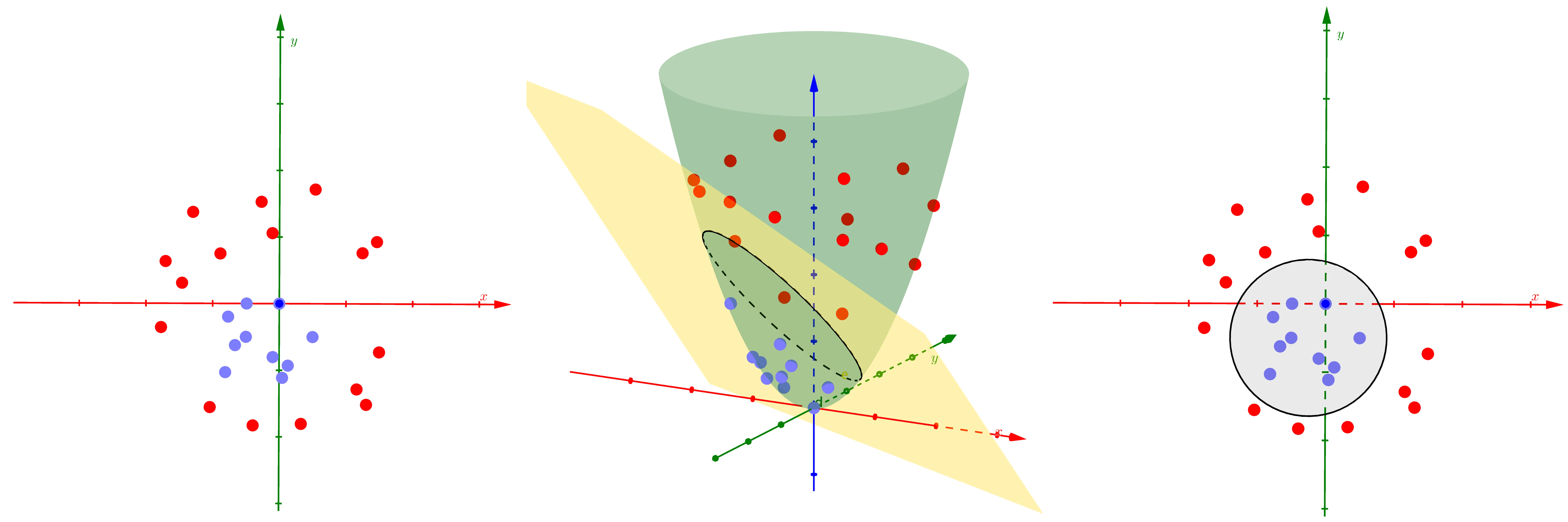
SVM can be employed for non-linear data by leveraging kernel functions and the kernel trick. Non-linear data are cases where we cannot separate the data with just a simple linear hyperplane without significant misclassification, we can observe the following example:

As we can see, on the left side is a dataset in $\mathbb{R}^2$ where a separating hyperplane (a line in this case) will perform horrible in separating the 2 classes. On a high level, the motivation for the kernel SVM model is that it projects the original data to a higher dimension space where the data is nearly linearly separable, after which the performance of said SVM is similar to a soft margin SVM model. In the middle, we can see that in this higher dimension space, the model still separate the data with a hyperplane (a plane in said space). On the right, after projecting back to the original dimension of the dataset, the boundaries are non-linear and will allow us to handle such non-linear data.

Kernel Function and Kernel Trick

Note that in $(7)$, we have:

$$\begin{gather*} \max_{\boldsymbol{\alpha}} \sum^N_{i=1} \alpha_i - \frac{1}{2} \alpha_i \alpha_j y_i y_j \mathbf{x}_i^\top \mathbf{x}_j \quad \\ \text{subject to:} \quad 0 \leq \alpha_i \leq C, \forall i \quad ; \quad \sum^N_{i=1} \alpha_i y_i = 0 \quad (7) \quad \end{gather*}$$

Block

We see that the optimization process only depends on the inner product $\mathbf{x}_i^\top \mathbf{x}_j$. This observation is crucial to introduce the concept of kernel functions. Let $\phi (\mathbf{x})$ be a function where:

$$\phi: \mathbf{R}^n \to \mathbf{R}^k,\quad \phi(\mathbf{x}) = (\phi_1(\mathbf{x}), \phi_2(\mathbf{x}), \ldots, \phi_k(\mathbf{x})), \quad k \in \mathbb{N} \text{ or } k = \infty$$

Block

Utilizing this arbitrary $\phi (\mathbf{x})$ function, our problem in $(7)$ becomes:

$$\begin{gather*} \max_{\boldsymbol{\alpha}} \sum^N_{i=1} \alpha_i - \frac{1}{2} \alpha_i \alpha_j y_i y_j \phi(\mathbf{x}_i)^\top \phi(\mathbf{x}_j) \quad \\ \text{subject to:} \quad 0 \leq \alpha_i \leq C, \forall i \quad ; \quad \sum^N_{i=1} \alpha_i y_i = 0 \quad (8) \quad \end{gather*}$$

Block

Due to $\phi (\mathbf{x})$ being able to project to $k \in \mathbb{N} \cup \{\infty\}$ dimensions, directly calculating $\phi (\mathbf{x})$ can prove expensive or even impossible. To resolve this, note how in $(8)$, the optimization still only depends on only the inner product $\phi(\mathbf{x}_i)^\top \phi(\mathbf{x}_j)$. Thus, if we are able to find a function $K(\mathbf{x}_i, \mathbf{x}_j)$ such that:

$$K(\mathbf{x}_i, \mathbf{x}_j) = \phi(\mathbf{x}_i)^\top \phi(\mathbf{x}_j) \quad$$

Block

Then explicitly calculating $\phi(\mathbf{x})$ is unnecessary. The function $K(\mathbf{x}_i, \mathbf{x}_j)$ is called a kernel function that can be defined by the user and must follow a few traits like symmetry, continuous, positive-semi definite and the Mercer inequality. The process of only calculating $K(\mathbf{x}_i, \mathbf{x}_j)$ and not $\phi(\mathbf{x})$ explicitly is called the kernel trick.

A few common kernel functions:

• Linear Kernel:

$$K(\mathbf{x}_i, \mathbf{x}_j) = \mathbf{x}_i^\top \mathbf{x}_j \quad$$

Block

• Polynomial Kernel:

$$K(\mathbf{x}_i, \mathbf{x}_j) = (\gamma\mathbf{x}_i^\top \mathbf{x}_j + r)^d \quad$$

Block

Where $\gamma$, $r$ and $d$ are hyperparameters defined by the user.

• Radial Basis Function (RBF Kernel) / Gaussian Kernel:

$$K(\mathbf{x}_i, \mathbf{x}_j) = \exp{\left(-\gamma\|\mathbf{x}_i - \mathbf{x}_j\|^2_2\right)} \quad$$

Block

Where $\gamma > 0$ is hyperparameters defined by the user.

• Sigmoid Kernel:

$$K(\mathbf{x}_i, \mathbf{x}_j) = \tanh(\gamma\mathbf{x}_i^\top \mathbf{x}_j + r) \quad$$

Block

Where $\gamma$ and $r$ are hyperparameters defined by the user.

Building the Optimization Problem

With the addition of kernel functions, the optimization problem in $(8)$ will become:

$$\begin{gather*} \max_{\boldsymbol{\alpha}} \sum^N_{i=1} \alpha_i - \frac{1}{2} \alpha_i \alpha_j y_i y_j K(\mathbf{x}_i, \mathbf{x}_j) \quad \\ \text{subject to:} \quad 0 \leq \alpha_i \leq C, \forall i \quad ; \quad \sum^N_{i=1} \alpha_i y_i = 0 \quad (9) \quad \end{gather*}$$

Block

Similar to hard and soft margin SVM, we can solve $(8)$ with quadratic solvers. Note that we cannot solve kernel SVM with gradient descent anymore, a limitation that often leads to kernel SVM having exponentially longer training and inference time as data grows.

Final Model

Instead of $\mathbf{w}$ and $b$, kernel SVM directly use the Lagrange multipliers found by the quadratic solver to create prediction for query point $\mathbf{x}_q$:

$$y_q = \text{sign}\left( \sum^N_{i=1} \alpha_i y_i K(\mathbf{x}_i, \mathbf{x}_q) \right) \quad$$

Block

Extra: SVM for Multiclass Classification

For multiclass classification with $K$ classes, there are 2 main approaches:

• One-vs-One: Will create $\frac{K(K-1)}{2}$ binary SVM models.
• One-vs-Rest: Will create $K$ binary SVM models.

References

• Chapter 9: Support Vector Machines - Wenjing Liao
• Support Vector Machines – An Introduction - Vojislav Kecman
• A Tutorial on Support Vector Machines for Pattern Recognition - Christopher J.C. Burges
• Lagrangian Duality for Dummies - David Knowles
• Support vector machines - Alessia Mammone, Marco Turchi and Nello Cristianini
• Support Vector Machines Explained - Tristan Fletcher