Table of Content

• Table of Content
• Multinomial Logistic Regression
• Binary Logistic Regression

Block

Multinomial Logistic Regression

Given dataset $X = \{ (x_i, y_i) \}_{i=1}^N$ where $x_i \in \mathbb{R}^n$ and $y_i \in \{ 1,2,\ldots,C \}$, the Multinomial Logistic Regression model states that the likelihood of the input $x$ belonging to class $y=c$ is:

$$P(y = c \mid x, \Theta, \mathcal{B}) = \frac{\exp(z_c)}{\sum^C_\kappa \exp(z_\kappa)} \space ; \quad z_\kappa = x^T \theta_\kappa + \beta_\kappa \quad$$

Block

• Where $\Theta = \{ \theta_1, \theta_2, \ldots, \theta_C \}$ are the weights and $\mathcal{B} = \{ \beta_1, \beta_2, \ldots, \beta_C \}$ are the biases and they make up the model’s parameters.
• The set $Z = \{ z_1, z_2, \ldots, z_C \}$ are called the logits for each of the $C$ classes, which contains the linear combinations of the input $x$ with the weights and biases.
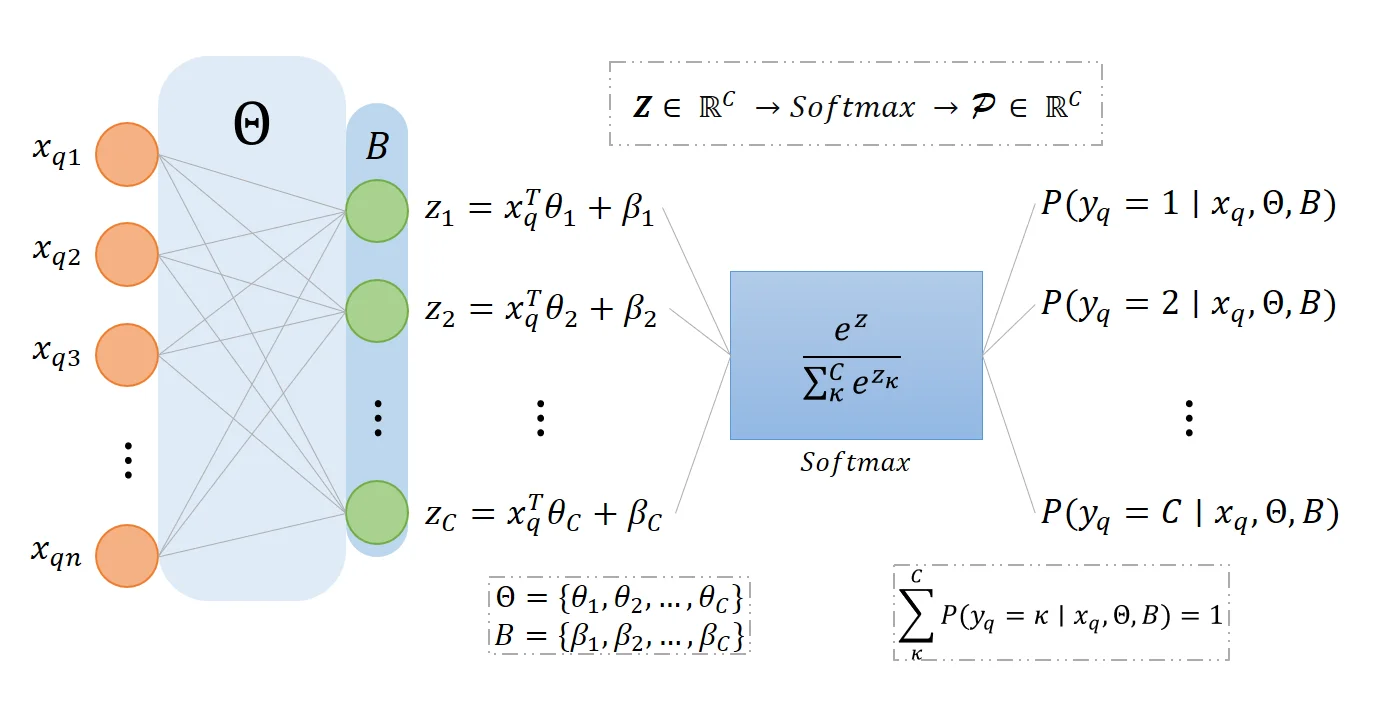
• The expression $\frac{\exp(z_c)}{\sum^C_\kappa \exp(z_\kappa)}$ is the $c$-th element of $\mathcal{P} = \{ P(y=1 \mid x, \Theta, \mathcal{B}), \ldots, P(y=C \mid x, \Theta, \mathcal{B}) \}$ produced by the Softmax Function, in nature it maps the $C$ linear combinations $Z$ of the input $x$ and the weights $\Theta$ and biases $\mathcal{B}$ to a probability distribution that sums up to 1. In other word, the softmax function takes $Z \in \mathbb{R}^C$ and produces $\mathcal{P} \in \mathbb{R}^C$ such that $\sum_c^C P(y=c \mid x, \Theta, \mathcal{B}) = 1$.

Here is a visualization of the multinomial logistic regression model in the style of a neural network for queried input $x_q$:

Our goal is to optimize the parameters $\Theta$ and $\mathcal{B}$, given MLE equation:

$$L(\Theta, \mathcal{B}) = \prod^N_{i=1} \prod^C_{c=1} \left( \frac{\exp(x_i^T \theta_c + \beta_c)}{\sum_{\kappa=1}^C \exp(x_i^T \theta_\kappa + \beta_\kappa)} \right)^{1[y_i=c]} \quad$$

Block

• Where $1[y_i=c]$ is an indicator function that equals 1 if $y_i = c$ and 0 otherwise.

We take the Log Likelihood to simplify the calculation of MLE:

$$\begin{gather*} \log L(\Theta, \mathcal{B}) = \sum^N_{i=1} \sum_{c=1}^C 1[y_1=c] \log \left( \frac{\exp(x_i^T \theta_c + \beta_c)}{\sum_{\kappa=1}^C \exp(x_i^T \theta_\kappa + \beta_\kappa)} \right) \quad \\[15pt] = \sum^N_{i=1} \sum_{c=1}^C 1[y_1=c] \left( x_i^T \theta_c + \beta_c - \log \left( \sum_{\kappa=1}^C \exp(x_i^T \theta_\kappa + \beta_\kappa) \right) \right) \quad \end{gather*}$$

Block

To maximize the MLE, we maximize the Log Likelihood, which is equivalent to minimizing the negative Log Likelihood, thus we define the cost function:

$$\begin{gather*} J(\Theta, \mathcal{B}) = -\frac{1}{N} \log L(\Theta, \mathcal{B}) \end{gather*}$$

Block

We use Gradient Descent to solve the optimization problem iteratively:

• Step 1: Initialize parameters randomly: $\Theta, \mathcal{B}$.
• Step 2: Calculate the Gradient of $J(\Theta, \mathcal{B})$ with respect to each of the logit’s weights $\theta_c$ and biases $\beta_c$:

$$\begin{gather*} \frac{\partial J}{\partial \theta_c} = -\frac{1}{N} \sum_{i=1}^N \left(1[y_i=c] - \frac{\exp(x_i^T \theta_c + \beta_c)}{\sum_{\kappa=1}^C \exp(x_i^T \theta_\kappa + \beta_\kappa)}\right)x_i \quad \\[15pt] \frac{\partial J}{\partial \beta_c} = -\frac{1}{N} \sum_{i=1}^N \left(1[y_i=c] - \frac{\exp(x_i^T \theta_c + \beta_c)}{\sum_{\kappa=1}^C \exp(x_i^T \theta_\kappa + \beta_\kappa)}\right) \end{gather*}$$

Block

These gradients will give us the direction of the weights and biases that will cause the steepest descent towards a local minima.

• Step 3: Update parameters:

$$\begin{gather*} \theta_c^{\text{new}} = \theta_c + \alpha \frac{\partial J}{\partial \theta_c} \quad \\[15pt] \beta_c^{\text{new}} = \beta_c + \alpha \frac{\partial J}{\partial \beta_c} \end{gather*}$$

Block

Where $\alpha$ denotes the learning rate. We perform step 2 and 3 for all logits from $1$ to $C$.

Often times, regularization is introduced to reduce overfitting, we will focus on L2 regularization, we implement it by simply adding a regularization term into the cost function:

$$J_{\text{reg}}(\Theta, \mathcal{B}) = -\frac{1}{N} \log L(\Theta, \mathcal{B}) + \frac{\lambda}{2N} \sum_{c=1}^C \| \theta_c \|^2_2 \quad$$

Block

Where $\lambda$ is a constant that represents the regularization strength. This will affect the weights of the model, large $\lambda$ causes the weights to be closer to 0 and needs to be tune strategically to properly reduce overfitting. While the biases updates remain unchanged, our weights updates will be affected:

$$\theta_c^{\text{new}} = \theta_c + \alpha \frac{\partial J}{\partial \theta_c} - \frac{\lambda}{N} \theta_c \quad$$

Block

Binary Logistic Regression

When there are $C = 2$ classes, the softmax function is reduced to a special case called the Sigmoid Function, for simplicity we let $y_i \in \{ 0, 1 \}$:

$undefined\; not\; callable\; (property\; \text{'}fill\text{'}\; of\; [object\; Array])$

Block

Let $\theta^{'} = \theta_2 - \theta_1$ and $\beta^{'} = \beta_2 - \beta_1$, we have:

$$\frac{1}{1+\exp(-(x_i^T \theta^{'} + \beta^{'}))} \space ; \quad 1 - \frac{1}{1+\exp(-(x_i^T \theta^{'} + \beta^{'}))}$$

Block

Which denotes the probability of class 0 and 1 respectively, notice that both of the expressions above still sum up to 1. Therefore, when $C = 2$, we only have to optimize for 1 set of weights $\theta^{'}$ and a single bias $\beta^{'}$. Given dataset $X = \{ (x_i, y_i) \}_{i=1}^N$ where $x_i \in \mathbb{R}^n$ and $y_i \in \{ 0,1\}$, the Binary Logistic Regression model or simply Logistic Regression model is represented as:

$$P(y \mid x, \theta, \beta) = (\sigma(z))^y(1-\sigma(z))^{1-y} \space ; \quad z = x^T\theta^{'} + \beta^{'} \quad$$

Block

• Where the weights $\theta^{'} = \{\theta_1, \theta_2, \ldots, \theta_n\}$ and bias $\beta^{'} \in \mathbb{R}$ are the model’s parameters.
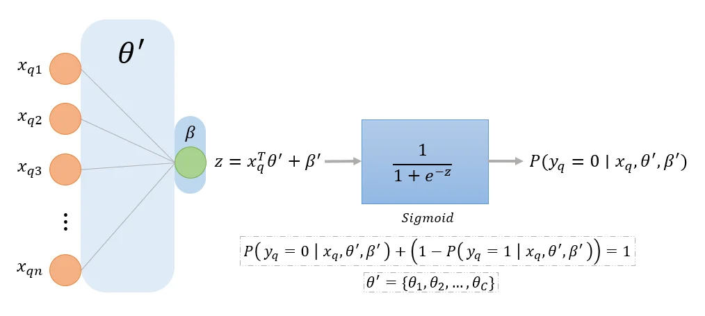
• The expression $\sigma(z) = \frac{1}{1+\exp(-z)}$ denotes the sigmoid function, and $z = x^T\theta^{'} + \beta^{'}$ denotes a linear combination of the input $x$ and the weights and bias, this function tends to $0$ as $z \rightarrow -\infty$ and tends to $1$ as $z \rightarrow +\infty$, and $\sigma(z) + (1-\sigma(z)) = 1$.

Here is a visualization of the binary logistic regression model in the style of a neural network for queried input $x_q$:

Our calculations will look a bit different:

• MLE:

$$L(\theta^{'}, \beta^{'}) = \prod_{i=1}^N P(y_i \mid x_i, \theta^{'}, \beta^{'}) \quad$$

Block

• Log Likelihood:

$$\log L(\theta^{'}, \beta^{'}) = \sum_{i=1}^N [y_i \log \sigma (z_i) + (1 - y_i) \log (1 - \sigma(z))] \quad$$

Block

• Cost function:

$$J(\theta^{'}, \beta^{'}) = - \frac{1}{N} \log L(\theta^{'}, \beta^{'}) \quad$$

Block

• Gradient Descent:

$$\begin{gather*} \frac{\partial J}{\partial \theta^{'}} = -\frac{1}{N} \sum_{i=1}^N (\sigma (z_i)- y_i)x_i \quad \\[10pt] \frac{\partial J}{\partial \beta^{'}} = -\frac{1}{N} \sum_{i=1}^N (\sigma (z_i)- y_i) \\[10pt] \theta^{'\text{ new}} = \theta^{'} + \alpha \frac{\partial J}{\partial \theta^{'}} \\[10pt] \beta^{'\text{ new}} = \beta^{'} + \alpha \frac{\partial J}{\partial \beta^{'}} \end{gather*}$$

Block

• L2 Regularization:

$$\begin{gather*} J_{\text{reg}} (\theta^{'}, \beta^{'}) = -\frac{1}{N} \log L(\theta^{'}, \beta^{'}) + \frac{1}{2N} \| \theta^{'} \|^2_2 \quad \\[10pt] \theta^{'\text{ new}} = \theta^{'} + \alpha \frac{\partial J}{\partial \theta^{'}} + \frac{1}{N} \theta^{'} \end{gather*}$$

Block