Logistic Regression - Python implementation from scratch

#machine-learning #python

30/09/2024 46 Min.

Written by: Yuk

Table of Content

Prologue

One of my biggest revelations in understanding logistic regression is to think of it as analogous to a neuron in a neural network. The linear combination in the forward pass, the non-linear activation function, and the application of gradient descent all mirror the components of a neural network. I must admit that this insight was a significant leap in my comprehension of the algorithm. It may seem unconventional to approach it from this angle, but recognizing that logistic regression serves as a fundamental building block for neural networks has been enlightening.

Having previously constructed a neural network from scratch in Java makes this algorithm particularly special to me, which is why this realization feels so personal. Initially, I was daunted by the complex mathematics and the intimidating nature of gradient descent, making me feel as though I was facing something entirely unfamiliar. However, as I’ve learned, when you find yourself struggling, seeking a new perspective—whether forward or, like me, backward—can lead to a deeper understanding. In the end, every effort to learn pays off.

This post will include:

✅ Python Implementation.

✅ Examples with Visualization.

✅ Brief and Concise explanation.

I, Overview

1. Logistic Regression

Logistic regression is a statistical method used for binary classification, predicting the probability that a given input belongs to one of two categories. It models the relationship between a dependent binary variable and one or more independent variables by applying the logistic function, which outputs values between 0 and 1. The model estimates the likelihood of an event occurring by transforming a linear combination of the input features using the logistic function.

In logistic regression, the coefficients are determined using maximum likelihood estimation (MLE), which finds the parameter values that make the observed data most probable. While traditional logistic regression focuses on binary outcomes, it can be extended to handle multiclass classification through techniques such as the one-vs-rest (OvR) approach and softmax regression.

The one-vs-rest approach treats each class as a separate binary classification problem, training a distinct model for each class to predict whether a given instance belongs to that class or not. On the other hand, softmax regression (Multinomial Logistic Regression) generalizes logistic regression to multiple classes by using the softmax function to convert the linear combinations of input features into a probability distribution across all classes.

This technique is widely used in various fields, including medicine, finance, and social sciences, for tasks like predicting disease presence, credit risk assessment, and customer behavior analysis.

2. Limitation of this Post

We will only cover Stochastic Gradient Descent (SGD) and the Newton-Raphson method for this implementation, you can look into more optimization algorithms such as Adam, Coordinate Descent, etc…
Assumption of linearity and balanced datasets: In reality, the nature of the data could be detrimental to linear models performance, for simplicity sake, we will only work on and give examples with datasets that suits logistic regression with the acknowledgement of its limitation.
We won’t go too in depth into the issue of Overfitting and Underfitting of logistic regression in this post.
This post will focus primarily on the coding aspects of logistic regression, providing practical implementations with minimal mathematical context. The theoretical foundations and detailed mathematical explanations will be covered in a future post.
Will only implement: Binary Logistic Regression with Sigmoid, Multiclass Logistic Regression with One vs. Rest approach or Softmax Regression (Multinomial Logistic Regression).

3. Necessary Imports

Throughout this post, we will assume these imports

import numpy as np  # For numerical operations and array manipulations.
import pandas as pd  # For data manipulation and analysis, especially with DataFrames.
import seaborn as sns # Specifically for heatmaps, which will be useful for multiclass evaluation.
import matplotlib.pyplot as plt  # For creating visualizations to help understand our data and results.

We will also use scikit-learn a lot for references so keep that in mind.

4. General process of Logistic Regression

Initialization: Begin by initializing the model parameters (weights and bias). These parameters can be set to small random values or zeros.
Forward Pass: Compute the linear combination of the input features using the initialized weights and bias.
Activation Function: Apply the logistic (sigmoid) function to the linear combination to obtain predicted probabilities.
Loss Calculation: Calculate the loss using a suitable loss function. For binary classification, the binary cross-entropy loss is commonly used, measuring the difference between predicted probabilities and true labels.
Optimization: Use an optimization algorithm (such as Stochastic Gradient Descent or the Newton-Raphson method) to update the model parameters. The goal is to minimize the loss function by adjusting the weights and bias iteratively based on the gradients computed from the loss.
Convergence Check: After updating the parameters, check for convergence by assessing whether the changes in the loss function or the parameters are below a specified threshold or whether the maximum number of iterations has been reached.
Prediction: Once the model is trained, make predictions on new data by following the forward pass and activation function steps. For binary classification, classify the output as 1 if the predicted probability is greater than 0.5, otherwise classify it as 0.
Multiclass Handling (if applicable): For multiclass classification, implement the one-vs-rest strategy or softmax regression, applying the same steps as above but ensuring that predictions account for multiple classes. For softmax, calculate probabilities for each class using the softmax function, and predict the class with the highest probability.

5. Final Goal of this Post

The aim of this journey is to implement a versatile logistic regression function that handles both binary and multiclass classification tasks. Here’s the plan:

def logistic_regression_predict(X_train, y_train, X_test, max_iter=10000, learning_rate=0.05, type='binary', regularization=None, reg_lambda=0.01):
    """Logistic Regression Prediction (Binary or Multiclass).

    This function predicts the output for a given test set using logistic regression.
    It supports both binary and multiclass classification based on the `type` parameter.

    Parameters:
        X_train: numpy.ndarray
            A 2D array of shape [m_samples, n_features] containing the training samples.
            Each row represents a sample and each column represents a feature.

        y_train: numpy.ndarray
            A 1D array of shape [m_samples] containing the training labels (0 or 1 for binary,
            or integer labels for multiclass). The length of this array must match the number of rows in X_train.

        X_test: numpy.ndarray
            A 2D array of shape [m_samples, n_features] containing the test samples to predict.
            It should have the same number of features as X_train.

        max_iter: int, optional
            The maximum number of iterations for the gradient descent algorithm to converge (default is 10000).
            Higher values may lead to better convergence but increase computation time.

        learning_rate: float, optional
            The step size used in the gradient descent update rule (default is 0.05).
            Smaller values may lead to more stable convergence but require more iterations.

        type: str, optional
            Determines the type of logistic regression problem (default is 'binary').
            Options include:
                - 'binary': Performs binary classification using sigmoid.
                - 'softmax': Explicitly performs multiclass classification using softmax regression (multinomial logistic regression).

        regularization: str or None, optional
            The type of regularization to apply (default is None).
            Options include:
                - 'l1': Lasso regularization (can lead to sparsity in model coefficients).
                - 'l2': Ridge regularization (helps prevent overfitting).
                - None: No regularization applied.

        reg_lambda: float, optional
            Parameter for regularization, can be ignored if regularization=None

    Returns:
        numpy.ndarray
            A 1D array of predicted labels for the test samples, with shape [m_samples].
            The output labels will be either binary (0 or 1) or class labels (0, 1, 2, ..., n_classes-1) 
            depending on the classification type (binary or multiclass).
    """
    return np.array(y_pred)

So without further ado, let’s get cooking.

II, Building the Model

In this section, we aim to implement three types of logistic regression: Binary Logistic Regression, One vs. Rest (OvR) classification, and Softmax Regression. Given the complexity involved, this discussion will be more extensive than our previous exploration of K-Nearest Neighbors (K-NN). To ensure a comprehensive understanding, we will present individual, standalone implementations for each of these models. Once we have developed a solid grasp of the intuition and mechanics behind each approach, we will integrate them into a cohesive and flexible function capable of handling both binary and multiclass classification tasks.

Additionally, due to the increased complexity of logistic regression, the explanation will be incredibly brief—as I do plan to cover them more in depth for my overview post on logistic regression.

1, Binary Logistic Regression

Binary Logistic Regression is a fundamental model for binary classification, predicting the probability that an input belongs to one of two classes. It uses a logistic function to convert a linear combination of features into a value between 0 and 1. Its simplicity makes it easier to interpret than more complex models like Softmax Regression, serving as a foundational building block for the One vs. Rest (OvR) approach. The OvR method applies multiple binary classifiers to handle multiclass problems effectively. In this section, we will implement Binary Logistic Regression from scratch and validate its functionality.

A. Sigmoid (Logit Function)

The sigmoid function maps any real-valued number to a value between 0 and 1, making it ideal for modeling probabilities. By applying the logistic function, we can interpret the output of our model as the probability that an input belongs to the positive class. We will also clip the input to avoid the risk of overflowing considering the presence of the exponential, this will help us ensure numerical stability in our calculation.

def sigmoid(z):
    z = np.clip(z, -500, 500)
    return 1 / (1 + np.exp(-z))

B. Prediction Function

The forward function calculates the predicted probabilities based on the current weights and input features. Including the intercept term (bias) allows the model to fit the data more flexibly (this is a common practice for linear models). The linear combination of weights and features, followed by the sigmoid activation, transforms this linear prediction into a probability.

def forward(weights, x):
    # Add bias term (column of 1s) to the input features
    x_with_bias = np.c_[np.ones(x.shape[0]), x]

    # Compute the linear combination of inputs and weights
    z = np.dot(x_with_bias, weights)

    # Apply the sigmoid function to get the predicted probabilities
    return sigmoid(z)

C. Loss Function (Log Loss / Cross-entropy)

The log_loss function quantifies the difference between predicted probabilities and actual class labels. By penalizing incorrect predictions more heavily, it provides a robust metric for evaluating model performance. Clipping predictions prevents taking the logarithm of zero, which would result in undefined values.

def log_loss(y_true, y_pred):
    # Clip predictions to avoid log(0)
    y_pred = np.clip(y_pred, 1e-15, 1 - 1e-15)
    return -np.mean(y_true * np.log(y_pred) + (1 - y_true) * np.log(1 - y_pred))

D. Update Weights

The update_weights function performs the core of the learning process. It calculates the error between predicted and true values, computes the gradient of the loss with respect to the weights, and updates the weights in the direction that reduces the loss. This iterative process gradually optimizes the model.

def update_weights(weights, x, y, learning_rate):
    # Forward pass
    y_pred = forward(weights, x)

    # Compute the error (gradient of loss w.r.t. predictions)
    error = y_pred - y

    # Compute gradient (with respect to weights)
    gradient = np.dot(np.c_[np.ones(x.shape[0]), x].T, error) / x.shape[0]

    # Update weights
    weights -= learning_rate * gradient
    return weights

E. Training Setup

The train function orchestrates the training process over multiple epochs using Stochastic Gradient Descent (SGD). By updating weights for each individual sample, it ensures thorough learning from the data. The optional log loss calculation at regular intervals allows for monitoring the model’s performance throughout training, providing insights into convergence.

# Using Stochastic Gradient Descent (SGD)
def train(weights, x, y, learning_rate, epochs):
     for epoch in range(epochs):
        # Iterate through each training sample
        for i in range(len(y)):
            # Update weights using the current sample
            weights = update_weights(weights, x[i:i+1], y[i:i+1], learning_rate)
        # Optional: Print log loss every 10 epochs
        # if epoch % 10 == 0:
        #     y_pred = forward(weights, x)
        #     loss = log_loss(y, y_pred)
    return weights

F. Proper Weights Initialization

The initialize_weights function sets the initial weights randomly. Proper initialization is crucial for effective training; it helps to break symmetry and encourages the model to explore various solutions. Including the bias term allows the model to shift the decision boundary appropriately.

def initialize_weights(input_dim):
    return np.random.randn(input_dim + 1)  # +1 for the bias term

G. Final Model

The binary_logistic_regression_predict function encapsulates the entire workflow of the Binary Logistic Regression model. It initializes the weights, trains the model using the training dataset, and then makes predictions on the test set.

def binary_logistic_regression_predict(X_train, y_train, X_test, max_iter=10000, learning_rate=0.05):
    # Initialize weights
    weights = initialize_weights(X_train.shape[1])

    # Train the model
    weights = train(weights, X_train, y_train, learning_rate, max_iter)

    # Make predictions on test set
    y_pred_probs = forward(weights, X_test)

    # Convert probabilities to binary predictions (0 or 1)
    y_pred = (y_pred_probs >= 0.5).astype(int)

    return np.array(y_pred)

2, One vs. Rest Logistic Regression

One vs. Rest (OVR) is a strategy used in multi-class classification problems. It involves training a separate binary classifier for each class, where that class is considered positive and all other classes are considered negative. The classifier that predicts the highest probability is chosen as the predicted class. This is essentially just leveraging the binary logistic regression model so this section would only serve as an extra to our final model which will use our binary and softmax logistic regression models as the final implementation

A. From Binary to Multiclass Classification

The function ovr_logistic_regression_predict provides a framework for handling multiclass classification by utilizing the concepts established in binary logistic regression. It effectively integrates the ability to recognize all unique labels within the dataset.

def ovr_logistic_regression_predict(X_train, y_train, X_test, max_iter=10000, learning_rate=0.05):
    num_classes = len(np.unique(y_train))  # Determine the number of unique classes
    predictions = np.zeros((X_test.shape[0], num_classes))  # Initialize predictions array

    # Train a binary classifier for each class
    for i in range(num_classes):
        # Create binary target labels for the current class
        binary_y_train = (y_train == i).astype(int)

        # Initialize weights for the binary classifier
        weights = initialize_weights(X_train.shape[1])

        # Train the binary logistic regression model
        weights = train(weights, X_train, binary_y_train, learning_rate, max_iter)

        # Predict probabilities for the test set using the trained model
        predictions[:, i] = forward(weights, X_test)

    # Select the class with the highest predicted probability for each test sample
    return np.argmax(predictions, axis=1)

In this implementation, the function is structured with clear, step-by-step calls to the necessary processes, facilitating the creation of a robust multiclass model. To enhance this, we can leverage our previous implementation by introducing a modified version of the binary_logistic_regression_predict_proba function:

def binary_logistic_regression_predict_proba(X_train, y_train, X_test, max_iter=10000, learning_rate=0.05):
    # Initialize weights
    weights = initialize_weights(X_train.shape[1])

    # Train the model
    weights = train(weights, X_train, y_train, learning_rate, max_iter)

    # Make predictions on test set as probabilities between 0 and 1
    y_pred_probs = forward(weights, X_test)

    return np.array(y_pred_probs)

Next, we can establish another version of ovr_logistic_regression_predict, which integrates both of our implementations seamlessly:

def ovr_logistic_regression_predict(X_train, y_train, X_test, max_iter=10000, learning_rate=0.05):
    num_classes = len(np.unique(y_train))  # Determine the number of unique classes
    predictions = np.zeros((X_test.shape[0], num_classes))  # Initialize predictions array

    # Train a binary classifier for each class using the existing binary logistic regression function
    for i in range(num_classes):
        # Create binary target labels for the current class
        binary_y_train = (y_train == i).astype(int)

        # Use the binary logistic regression predictor to train the model and get predictions
        predictions[:, i] = binary_logistic_regression_predict_proba(X_train, binary_y_train, X_test,
                                                               max_iter=max_iter,
                                                               learning_rate=learning_rate)

    # Select the class with the highest predicted probability for each test sample
    return np.argmax(predictions, axis=1)

B. Logistic Regression Approaches to Multiclass Classification

Other than the One vs. Rest approach, we still have other types of practice to handle multiclass classification when leveraging the Binary Classification basis. Those include:

Hierarchical
One vs. One
One vs. Rest
Binary Coding

Because we won’t go too in depth into these concepts, here are a few illustration to help you get the intuition of these many approaches:

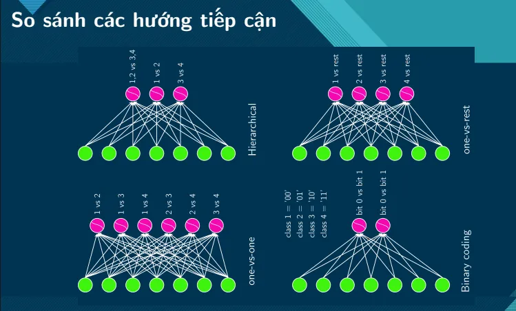
Multiclass Approaches of Logistic Regression

The many approaches of Logistic Regresion to Multiclass Classification

Translation: Comparing different approaches.

Multiclass Approaches of Logistic Regression

Suitable use case of each approaches

Translation: Understanding use case of each approaches.

Figure a, All 4 approaches are not viable.
Figure b, One vs. Rest is not applicable due to not being able to linearly separate class Green from other classes.
Figure c, Similar to figure b, can only apply One vs. One or Hierarchical. Potential solution: Use One vs. Rest on class Red (Red and non-Red), and class Blue and Yellow. The rest of the data can be separated with One vs. One or Hierarchical.

All content and Illustrations in this section belongs to Cao Van Chung - Multinomial Logistic Regresson (Softmax Regression).

3. Softmax Regression (Multinomial Logistic Regression)

Softmax Regression, also known as Multinomial Logistic Regression, extends binary logistic regression to handle multiple classes. It predicts the probabilities of each input belonging to one of several classes using the softmax function, ensuring that the outputs are valid probabilities that sum to one. This approach is commonly used in classification tasks where there are more than two possible outcomes, almost an extension of classic binary logistic regression.

A. Softmax

The softmax function converts the linear combination of features into a probability distribution across multiple classes. This transformation ensures that each output is a value between 0 and 1, with the sum of all outputs equal to 1, making it suitable for multiclass classification.

def softmax(z):
    z = np.clip(z, -500, 500)
    exp_z = np.exp(z)
    return exp_z / np.sum(exp_z, axis=1, keepdims=True)

B. Cross-Entropy Loss

The cross_entropy_loss function measures the performance of the model by quantifying the difference between the true class labels and predicted probabilities. By penalizing the model for incorrect predictions, it guides the optimization process to improve classification accuracy.

def cross_entropy_loss(y_true, y_pred):
    # Clip predictions to avoid log(0)
    y_pred = np.clip(y_pred, 1e-15, 1 - 1e-15)
    # Convert y_true to one-hot encoding if it is not
    y_one_hot = np.eye(y_pred.shape[1])[y_true]
    return -np.mean(np.sum(y_one_hot * np.log(y_pred), axis=1))

C. One-hot Encoding

One-hot encoding is used to represent the true class labels in a format suitable for comparing with the predicted probabilities. By converting each class label into a vector with a single “hot” (1) value, we can effectively calculate the error during training and apply updates to the model weights. We implement this in the following functions:

def cross_entropy_loss(y_true, y_pred):
    # Clip predictions to avoid log(0)
    y_pred = np.clip(y_pred, 1e-15, 1 - 1e-15)
    # Convert y_true to one-hot encoding if it is not
    y_one_hot = np.eye(y_pred.shape[1])[y_true]
    return -np.mean(np.sum(y_one_hot * np.log(y_pred), axis=1))

def update_weights(weights, x, y, learning_rate):
    # Forward pass
    y_pred = forward(weights, x)

    # Convert y to one-hot encoding
    y_one_hot = np.eye(y_pred.shape[1])[y]

    # Compute the error (gradient of loss w.r.t. predictions)
    error = y_pred - y_one_hot

    # Compute gradient (with respect to weights)
    gradient = np.dot(np.c_[np.ones(x.shape[0]), x].T, error) / x.shape[0]

    # Update weights
    weights -= learning_rate * gradient
    return weights

D. Final Model

The softmax_logistic_regression_predict function wraps the entire workflow of Softmax Regression. It initializes the weights, trains the model using a training dataset, and makes predictions on the test set. The output is the predicted class for each test sample, obtained by selecting the class with the highest probability.

def softmax_logistic_regression_predict(X_train, y_train, X_test, max_iter=10000, learning_rate=0.05):
    num_classes = len(np.unique(y_train))  # Determine the number of unique classes
    # Initialize weights
    weights = initialize_weights(X_train.shape[1], num_classes)

    # Train the model
    weights = train(weights, X_train, y_train, learning_rate, max_iter)

    # Make predictions on test set
    y_pred_probs = forward(weights, X_test)

    # Convert probabilities to class predictions (0, 1, ..., num_classes-1)
    y_pred = np.argmax(y_pred_probs, axis=1)

    return np.array(y_pred)

4. Regularization

Regularization is a technique used to prevent overfitting in logistic regression by adding a penalty to the model’s complexity, encouraging simpler models that generalize better.

L1 Regularization: Adds a penalty based on the absolute values of the model’s coefficients, leading to sparse solutions where some coefficients are reduced to zero. This helps in feature selection.
L2 Regularization: Adds a penalty based on the squared values of the coefficients, encouraging smaller values overall but rarely reducing them to zero. It helps distribute the influence across all features more evenly.

We will implement regularization into the logic of our models in the Final Result.

5. Final Result

By encapsulating our models into a single module, we can seamlessly work with them in our experiments and visualization, first let’s give a run down of our models so far after implementing regularization.

A. Binary Logistic Regression Model

The bin_log_reg.py module:

import numpy as np

def sigmoid(z):
    z = np.clip(z, -500, 500)
    return 1 / (1 + np.exp(-z))

def forward(weights, x):
    # Add bias term (column of 1s) to the input features
    x_with_bias = np.c_[np.ones(x.shape[0]), x]

    # Compute the linear combination of inputs and weights
    z = np.dot(x_with_bias, weights)

    # Apply the sigmoid function to get the predicted probabilities
    return sigmoid(z)

def log_loss(y_true, y_pred):
    # Clip predictions to avoid log(0)
    y_pred = np.clip(y_pred, 1e-15, 1 - 1e-15)
    return -np.mean(y_true * np.log(y_pred) + (1 - y_true) * np.log(1 - y_pred))

def update_weights(weights, x, y, learning_rate, regularization=None, reg_lambda=0.01):
    # Forward pass
    y_pred = forward(weights, x)

    # Compute the error (gradient of loss w.r.t. predictions)
    error = y_pred - y

    # Compute gradient (with respect to weights)
    gradient = np.dot(np.c_[np.ones(x.shape[0]), x].T, error) / x.shape[0]

    # Apply L1 or L2 regularization to the gradient (excluding bias term)
    if regularization == 'l2':
        gradient[1:] += reg_lambda * weights[1:] / x.shape[0]
    elif regularization == 'l1':
        gradient[1:] += reg_lambda * np.sign(weights[1:]) / x.shape[0]

    # Update weights
    weights -= learning_rate * gradient
    return weights

def train(weights, x, y, learning_rate, epochs, regularization=None, reg_lambda=0.01):
    for epoch in range(epochs):
        for i in range(len(y)):
            weights = update_weights(weights, x[i:i+1], y[i:i+1], learning_rate, regularization, reg_lambda)
        # Optional: Print log loss every 10 epochs
        # if epoch % 10 == 0:
        #     y_pred = forward(weights, x)
        #     loss = log_loss(y, y_pred)
    return weights

def initialize_weights(input_dim):
    return np.random.randn(input_dim + 1)  # +1 for the bias term

def binary_logistic_regression_predict(X_train, y_train, X_test, max_iter=10000, learning_rate=0.05, regularization=None, reg_lambda=0.01):
    # Initialize weights
    weights = initialize_weights(X_train.shape[1])

    # Train the model
    weights = train(weights, X_train, y_train, learning_rate, max_iter, regularization, reg_lambda)

    # Make predictions on test set
    y_pred_probs = forward(weights, X_test)

    # Convert probabilities to binary predictions (0 or 1)
    y_pred = (y_pred_probs >= 0.5).astype(int)

    return np.array(y_pred)

def binary_logistic_regression_predict_proba(X_train, y_train, X_test, max_iter=10000, learning_rate=0.05, regularization=None, reg_lambda=0.01):
    # Initialize weights
    weights = initialize_weights(X_train.shape[1])

    # Train the model
    weights = train(weights, X_train, y_train, learning_rate, max_iter, regularization, reg_lambda)

    # Make predictions on test set
    y_pred_probs = forward(weights, X_test)

    return np.array(y_pred_probs)

For completeness, we can utilized the regularized models of bin_log_reg.py to achieve the One vs. Rest approach which we gone through above. Below is the ovr_log_reg.py module, utilizing the bin_log_reg.py module:

from bin_log_reg.py import binary_logistic_regression_predict_proba

def ovr_logistic_regression_predict(X_train, y_train, X_test, max_iter=10000, learning_rate=0.05, regularization=None, reg_lambda=0.01):
    num_classes = len(np.unique(y_train))  # Determine the number of unique classes
    predictions = np.zeros((X_test.shape[0], num_classes))  # Initialize predictions array

    # Train a binary classifier for each class using the existing binary logistic regression function
    for i in range(num_classes):
        # Create binary target labels for the current class
        binary_y_train = (y_train == i).astype(int)

        # Use the binary logistic regression predictor to train the model and get predictions
        predictions[:, i] = binary_logistic_regression_predict_proba(
            X_train, binary_y_train, X_test,
            max_iter=max_iter,
            learning_rate=learning_rate,
            regularization=regularization,
            reg_lambda=reg_lambda
        )

    # Select the class with the highest predicted probability for each test sample
    return np.argmax(predictions, axis=1)

B. Softmax Regression Model

The softmax_log_reg.py module:

import numpy as np

def softmax(z):
    z = np.clip(z, -500, 500)
    exp_z = np.exp(z)
    return exp_z / np.sum(exp_z, axis=1, keepdims=True)

def forward(weights, x):
    # Add bias term (column of 1s) to the input features
    x_with_bias = np.c_[np.ones(x.shape[0]), x]

    # Compute the linear combination of inputs and weights
    z = np.dot(x_with_bias, weights)

    # Apply the softmax function to get the predicted probabilities
    return softmax(z)

def cross_entropy_loss(y_true, y_pred):
    # Clip predictions to avoid log(0)
    y_pred = np.clip(y_pred, 1e-15, 1 - 1e-15)
    # Convert y_true to one-hot encoding if it is not
    y_one_hot = np.eye(y_pred.shape[1])[y_true]
    return -np.mean(np.sum(y_one_hot * np.log(y_pred), axis=1))

def update_weights(weights, x, y, learning_rate, regularization=None, reg_lambda=0.01):
    # Forward pass
    y_pred = forward(weights, x)

    # Convert y to one-hot encoding
    y_one_hot = np.eye(y_pred.shape[1])[y]

    # Compute the error (gradient of loss w.r.t. predictions)
    error = y_pred - y_one_hot

    # Compute gradient (with respect to weights)
    gradient = np.dot(np.c_[np.ones(x.shape[0]), x].T, error) / x.shape[0]

    # Apply L1 or L2 regularization to weights (excluding bias term)
    if regularization == 'l1':
        gradient[1:] += reg_lambda * np.sign(weights[1:]) / x.shape[0]
    elif regularization == 'l2':
        gradient[1:] += reg_lambda * weights[1:] / x.shape[0]

    # Update weights
    weights -= learning_rate * gradient
    return weights

def train(weights, x, y, learning_rate, epochs, regularization=None, reg_lambda=0.01):
    for epoch in range(epochs):
        for i in range(len(y)):
            weights = update_weights(weights, x[i:i+1], y[i:i+1], learning_rate, regularization, reg_lambda)
        # Optional: Print cross-entropy loss every 10 epochs
        # if epoch % 10 == 0:
        #     y_pred = forward(weights, x)
        #     loss = cross_entropy_loss(y, y_pred)
    return weights

def initialize_weights(input_dim, num_classes):
    return np.random.randn(input_dim + 1, num_classes)  # +1 for the bias term

def softmax_logistic_regression_predict(X_train, y_train, X_test, max_iter=10000, learning_rate=0.05, regularization=None, reg_lambda=0.01):
    num_classes = len(np.unique(y_train))  # Determine the number of unique classes
    # Initialize weights
    weights = initialize_weights(X_train.shape[1], num_classes)

    # Train the model
    weights = train(weights, X_train, y_train, learning_rate, max_iter, regularization, reg_lambda)

    # Make predictions on test set
    y_pred_probs = forward(weights, X_test)

    # Convert probabilities to class predictions (0, 1, ..., num_classes-1)
    y_pred = np.argmax(y_pred_probs, axis=1)

    return np.array(y_pred)

C. Final Model

Now, with all the building block in place, we can finally combine them all into a coherent log_reg_model.py module which achieved our final goal of the logistic_regression_predict function. I’ve also modified initialize_weights to follow a normal distribution with seed control to ensure reproducibility. I’ve also added an early stop mechanism in the form of check_weight_convergence to ensure efficiency in cases where the model doesn’t converge beyond max_iter. The model can handle both binary and multiclass classification with inclusion of l1 and l2 regularization

import numpy as np

def sigmoid(z):
    z = np.clip(z, -500, 500)
    return 1 / (1 + np.exp(-z))

def softmax(z):
    z = np.clip(z, -500, 500)
    exp_z = np.exp(z)
    return exp_z / np.sum(exp_z, axis=1, keepdims=True)

def forward(weights, x, classification_type='binary'):
    # Add bias term (column of 1s) to the input features
    x_with_bias = np.c_[np.ones(x.shape[0]), x]

    # Compute the linear combination of inputs and weights
    z = np.dot(x_with_bias, weights)

    if classification_type == 'binary':
        return sigmoid(z)
    elif classification_type == 'softmax':
        return softmax(z)

def log_loss(y_true, y_pred):
    # Clip predictions to avoid log(0)
    y_pred = np.clip(y_pred, 1e-15, 1 - 1e-15)
    return -np.mean(y_true * np.log(y_pred) + (1 - y_true) * np.log(1 - y_pred))

def cross_entropy_loss(y_true, y_pred):
    # Clip predictions to avoid log(0)
    y_pred = np.clip(y_pred, 1e-15, 1 - 1e-15)
    # Convert y_true to one-hot encoding if it is not
    y_one_hot = np.eye(y_pred.shape[1])[y_true]
    return -np.mean(np.sum(y_one_hot * np.log(y_pred), axis=1))

def update_weights(weights, x, y, learning_rate, regularization=None, reg_lambda=0.01, classification_type='binary'):
    # Forward pass
    y_pred = forward(weights, x, classification_type)

    # Compute the error (gradient of loss w.r.t. predictions)
    if classification_type == 'binary':
        error = y_pred - y
    elif classification_type == 'softmax':
        y_one_hot = np.eye(y_pred.shape[1])[y]
        error = y_pred - y_one_hot

    # Compute gradient (with respect to weights)
    gradient = np.dot(np.c_[np.ones(x.shape[0]), x].T, error) / x.shape[0]

    # Apply L1 or L2 regularization to the gradient (excluding bias term)
    if regularization == 'l2':
        gradient[1:] += reg_lambda * weights[1:] / x.shape[0]
    elif regularization == 'l1':
        gradient[1:] += reg_lambda * np.sign(weights[1:]) / x.shape[0]

    # Update weights
    weights -= learning_rate * gradient
    return weights

def initialize_weights(input_dim, num_classes=1, seed=42):
    np.random.seed(seed)
    return np.random.normal(0, 1, (input_dim + 1, num_classes))

def check_weight_convergence(old_weights, new_weights, tolerance=1e-4):
    return np.all(np.abs(new_weights - old_weights) < tolerance)

def train(weights, x, y, learning_rate, epochs, regularization=None, reg_lambda=0.01, classification_type='binary'):
    old_weights = np.copy(weights)
    for epoch in range(epochs):
        for i in range(len(y)):
            weights = update_weights(weights, x[i:i+1], y[i:i+1], learning_rate, regularization, reg_lambda, classification_type)

        # Check for convergence every 20 iterations
        if (epoch + 1) % 20 == 0:
            if check_weight_convergence(old_weights, weights):
                # Uncomment the line below to know when the model converged
                # print(f"Converged after {epoch + 1} epochs")
                return weights
            old_weights = np.copy(weights)

        # Uncomment the following section to print the loss over epochs
        # y_pred = forward(weights, x, classification_type)
        # if classification_type == 'binary':
        #     loss = log_loss(y, y_pred)
        # elif classification_type == 'softmax':
        #     loss = cross_entropy_loss(y, y_pred)
        # print(f"Epoch {epoch + 1}/{epochs}, Loss: {loss:.4f}")

    # Uncomment the line below to know if the model reached maximum iteration count
    # print(f"Reached maximum number of epochs: {epochs}")
    return weights

def logistic_regression_predict(X_train, y_train, X_test, max_iter=10000, learning_rate=0.05, type='binary', regularization=None, reg_lambda=0.01):
    # Weight initialization
    if type == 'binary':
        weights = initialize_weights(X_train.shape[1])
    elif type == 'softmax':
        num_classes = len(np.unique(y_train))
        weights = initialize_weights(X_train.shape[1], num_classes)

    # Train the model
    weights = train(weights, X_train, y_train, learning_rate, max_iter, regularization, reg_lambda, type)

    # Make predictions on test set
    y_pred_probs = forward(weights, X_test, type)

    # Convert probabilities to class predictions
    if type == 'binary':
        y_pred = (y_pred_probs >= 0.5).astype(int)
    elif type == 'softmax':
        y_pred = np.argmax(y_pred_probs, axis=1)

    return np.array(y_pred)

III, Testing the Model

After finalizing our model, now it’s time to put it to the test. We will go over many examples, experiments and even stacking it up against the MNIST dataset—an image classification task, a problem that only seems some what viable thanks to logistic regression considering the models we have evaluated before (K-NN, Linear Regression).

1. Evaluation Metrics for Logistic Regression

Accuracy: Measures the proportion of correct predictions out of total predictions, indicating overall model performance.
Recall: Assesses the ability to correctly identify all relevant instances, useful for minimizing false negatives.
Precision: Evaluates the proportion of true positive predictions among all positive predictions, important for minimizing false positives.
F1-score: The harmonic mean of precision and recall, balancing the trade-off between false positives and false negatives.
Confusion Matrix: Summarizes the classification results, showing the counts of true and false positives/negatives.
Log Loss: Measures the performance by penalizing incorrect predictions with high confidence, indicating model uncertainty.

2. Visualization for Logistic Regression

Confusion Matrix Heatmap: Provides a visual representation of prediction performance across all classes, highlighting errors. This is especially useful for multiclass classification compared to standard confusion matrix.
Decision Boundary Plot: Shows how the model separates different classes in feature space, useful for visualizing model behavior.

3. Examples with Visualization

A. Studying Hours (Binary Logistic Regression)

Let’s start with a simple and familiar example: Study Hours vs. Test Results. The dataset expresses how student’s study hours will affect their test result (1 for Pass and 0 for Not Pass). We initialize the data, then use our logistic regression model with max_iter=50 with no regularization:

import numpy as np
from log_reg_model import logistic_regression_predict
from sklearn.model_selection import train_test_split
from sklearn.metrics import accuracy_score, precision_score, recall_score, confusion_matrix

# Initiating data
hours = np.array([0.50, 0.75, 1.00, 1.25, 1.50, 1.75, 1.75, 2.00, 2.25, 2.50,
                  2.75, 3.00, 3.25, 3.50, 4.00, 4.25, 4.50, 4.75, 5.00, 5.50])
pass_array = np.array([0, 0, 0, 0, 0, 0, 1, 0, 0, 0,
                       1, 0, 1, 0, 1, 1, 1, 1, 1, 1])

hours = hours.reshape(-1, 1)  # Reshape to 2D array

# Create training set and test set
X_train, X_test, y_train, y_test = train_test_split(hours, pass_array, train_size=15, test_size=5, random_state=42)

# Use our LogReg model
y_pred = logistic_regression_predict(X_train, y_train, X_test, max_iter=50, type='binary')

# Print out evaluation metrics
accuracy = accuracy_score(y_test, y_pred)
print("Accuracy:", accuracy)
precision = precision_score(y_test, y_pred)
print("Precision:", precision)
recall = recall_score(y_test, y_pred)
print("Recall:", recall)
conf_matrix = confusion_matrix(y_test, y_pred)
print("Confusion Matrix:\n", conf_matrix)

Accuracy: 1.0
Precision: 1.0
Recall: 1.0
Confusion Matrix:
 [[3 0]
 [0 2]]

You can see that our model performed perfectly on the test set, which indicates a strong start! These results are also in relation to how simple the dataset is—the data is easily separated by a linear approach. Now, to better visualize the results and even stack it up against new data, we can perform the following:

import numpy as np
import matplotlib.pyplot as plt
from sklearn.model_selection import train_test_split
from sklearn.metrics import accuracy_score, precision_score, recall_score, confusion_matrix

from final_model import logistic_regression_predict_proba # You simply don't convert them from probability to labels

# Initiating data
hours = np.array([0.50, 0.75, 1.00, 1.25, 1.50, 1.75, 1.75, 2.00, 2.25, 2.50,
                  2.75, 3.00, 3.25, 3.50, 4.00, 4.25, 4.50, 4.75, 5.00, 5.50])
pass_array = np.array([0, 0, 0, 0, 0, 0, 1, 0, 0, 0,
                       1, 0, 1, 0, 1, 1, 1, 1, 1, 1])

# Reshape for model
hours = hours.reshape(-1, 1)

# Create training set and test set
X_train, X_test, y_train, y_test = train_test_split(hours, pass_array, train_size=15, test_size=5, random_state=42)

# Prepare for plotting
new_study_hours = np.array([2.45, 1.85, 3.75, 3.21, 4.05])

# Plot original data
plt.figure(figsize=(10, 6))

# Original data points
plt.scatter(hours[pass_array == 0], np.zeros(sum(pass_array == 0)), color='blue', label='Not Pass (0)', alpha=0.6, edgecolors='k')
plt.scatter(hours[pass_array == 1], np.ones(sum(pass_array == 1)), color='red', label='Pass (1)', alpha=0.6, edgecolors='k')

# Prepare x values for the sigmoid curve
x_values = np.linspace(0, 5.5, 100).reshape(-1, 1)
# Get predictions (probabilities) for these x values
sigmoid_probs = logistic_regression_predict_proba(X_train, y_train, x_values, max_iter=50, type='binary')

# Plot the sigmoid decision boundary
plt.plot(x_values, sigmoid_probs, color='orange', label='Sigmoid Decision Boundary')

# Plot new study hours
new_probs = logistic_regression_predict_proba(X_train, y_train, new_study_hours.reshape(-1, 1), max_iter=50, type='binary')
plt.scatter(new_study_hours, new_probs, color='green', marker='D', label='New Study Hours', s=100)

# Highlight the threshold at y=0.5
plt.axhline(0.5, color='purple', linestyle='--', label='Threshold (0.5)')

# Formatting the plot
plt.xlim(0, 5.5)
plt.ylim(-0.1, 1.1)
plt.axhline(0, color='black', lw=0.5, ls='--')
plt.axhline(1, color='black', lw=0.5, ls='--')
plt.title('Study Hours vs Pass/Not Pass Decision Boundary')
plt.xlabel('Study Hours')
plt.ylabel('Probability')
plt.legend()
plt.grid(True)
plt.show()

Study Hours

Study Hours vs. Test Result

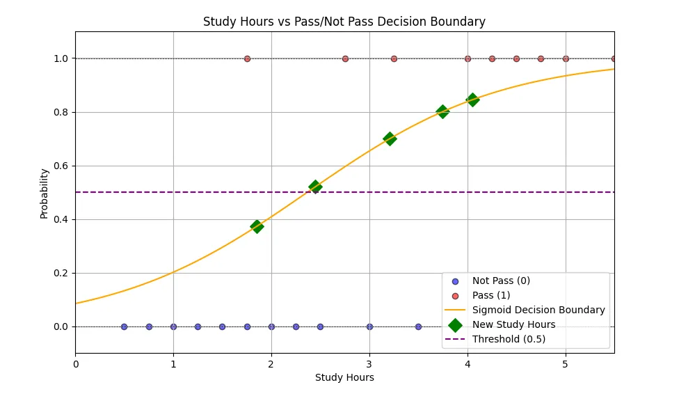
With the plot above, you can easily interpret the original data. As you can see, there are still many data points that “overlaps” (ie. Low study hours but still pass and vice versa). Yet our model was still able to capture their relationship and performed perfectly on the test set, this implies the usefulness of logistic regression even when the data doesn’t perfectly display a threshold. The plot also highlighted the Sigmoid function, which is exactly what logistic regression used to perform binary classification, we can see that the model predicted 4/5 new data points as Pass, which should be expected.

B. Graduate Admission (Binary Logistic Regression)

Dataset: Graduate-Admission-Prediction

Here, we consider the dataset above. Let’s give a run down of the characteristics of the data:

Graduate Record Exam (GRE): score. The score will be out of 340 points.
Test of English as a Foreigner Language (TOEFL): score, which will be out of 120 points.
University Rating (Uni.Rating): that indicates the Bachelor University ranking among the other universities. The score will be out of 5.
Statement of purpose (SOP): which is a document written to show the candidate’s life, ambitious and the motivations for the chosen degree/university. The score will be out of 5 points.
Letter of Recommendation Strength (LOR): which verifies the candidate professional experience, builds credibility, boosts confidence and ensures your competency. The score is out of 5 points
Undergraduate GPA (CGPA): out of 10
Research Experience: that can support the application, such as publishing research papers in conferences, working as research assistant with university professor (either 0 or 1).
Chance of Admit: Ranging from 0 to 1.

Note: The description is cited from the paper included in the dataset’s link.

This time around, we will need to engineer a target variable y as Chance of Admit is a float value raging from 0 to 1, indicating the probability of whether or not that student would be admit. We will add another column Admit to the data, which is defined as 1 if the Chance of Admit is \(\geq\) 0.7 and 0 otherwise. This choice is arbitrary and is purely personal preference.

We then use our model to predict on the test set (Original split ratio 8:2). Given the larger and more complex dataset, we use max_iter=1000 to ensure the chance of convergence in gradient descent:

import pandas as pd
from log_reg_model import logistic_regression_predict
from sklearn.model_selection import train_test_split
from sklearn.metrics import accuracy_score, precision_score, recall_score, confusion_matrix
from sklearn.preprocessing import StandardScaler

# Load the dataset
data = pd.read_csv('data/admission.csv')

# Add the target column 'Admit'
data['Admit'] = (data['Chance of Admit '] >= 0.7).astype(int)

# Drop unnecessary columns (like 'Serial No.' and 'Chance of Admit ')
data = data.drop(columns=['Serial No.', 'Chance of Admit '])

# Extract features (X) and target (y)
X = data.drop(columns=['Admit']).values
y = data['Admit'].values

# Split the data into training and test sets (80:20 split)
X_train, X_test, y_train, y_test = train_test_split(X, y, test_size=0.2, random_state=42)

# Train the model and make predictions on the test set
y_pred = logistic_regression_predict(X_train, y_train, X_test, max_iter=1000, learning_rate=0.05, type='binary')

# Calculate and print evaluation metrics
accuracy = accuracy_score(y_test, y_pred)
precision = precision_score(y_test, y_pred)
recall = recall_score(y_test, y_pred)
conf_matrix = confusion_matrix(y_test, y_pred)

print(f"Accuracy: {accuracy:.4f}")
print(f"Precision: {precision:.4f}")
print(f"Recall: {recall:.4f}")
print("Confusion Matrix:")
print(conf_matrix)

Accuracy: 0.5875
Precision: 1.0000
Recall: 0.3889
Confusion Matrix:
[[26  0]
 [33 21]]

After the initial model evaluation, we observed that our model did not perform well, achieving an accuracy of 0.5875—slightly above random guessing. While the model exhibited perfect precision (indicating that every instance it predicted as positive was indeed positive), it also demonstrated a low recall of 0.3889. This suggests that the model was conservative in its predictions of positive cases, leading to many missed true positives, as reflected in the confusion matrix.

To improve the model’s performance, we first addressed the varying scales of the features by applying normalization. Normalization helps ensure that the continuous features follow a standard scale, which is particularly crucial for linear models and higher-dimensional datasets. For this, we will use the StandardScaler of sklearn:

from sklearn.preprocessing import StandardScaler

# The same code above...

# Extract features (X) and target (y)
X = data.drop(columns=['Admit']).values
y = data['Admit'].values

# Normalize the features using StandardScaler
scaler = StandardScaler()
X = scaler.fit_transform(X)

# Split the data into training and test sets (80:20 split)
X_train, X_test, y_train, y_test = train_test_split(X, y, test_size=0.2, random_state=42)

# The same code below...

Accuracy: 0.8500
Precision: 0.8500
Recall: 0.9444
Confusion Matrix:
[[17  9]
 [ 3 51]]

After normalization, we retrained the model and observed a significant improvement in performance, achieving an accuracy of 0.8500, along with precision and recall scores of 0.8500 and 0.9444, respectively. The confusion matrix showed that the model was now capturing more true positive cases while still maintaining a reasonable number of false positives.

Next, we implemented regularization to further enhance model performance. To do this, we performed a Grid Search, which allows us to find the best-performing model by exploring a wide range of combinations of hyperparameters. We considered two types of regularization: l1 and l2, and varied the regularization strength, denoted as lambda, across several values.

# The same code above...

# Split the data into training and test sets (80:20 split)
X_train, X_test, y_train, y_test = train_test_split(X, y, test_size=0.2, random_state=42)

# Define the parameter grid
regularization_list = ['l1', 'l2']
reg_lambda_list = [0.01, 0.05, 0.1, 0.5, 1.0, 5.0, 10.0, 100.0]

# Variables to store the best model and its metrics
best_accuracy = 0
best_model_params = None
best_metrics = None

# Define constant parameters
default_iter = 1000
default_learning_rate = 0.05

# Perform grid search
print("Grid Search Results (Accuracy):")
print(f"{'Regularization':<15} {'Lambda':<10} {'Accuracy':<10}")
print("-" * 40)

for regularization in regularization_list:
    for reg_lambda in reg_lambda_list:
        # Train the model
        y_pred = logistic_regression_predict(
            X_train, y_train, X_test,
            max_iter=default_iter,
            learning_rate=default_learning_rate,
            type='binary',
            regularization=regularization,
            reg_lambda=reg_lambda
        )

        # Calculate accuracy
        accuracy = accuracy_score(y_test, y_pred)

        # Print the accuracy for the current combination
        print(f"{regularization:<15} {reg_lambda:<10} {accuracy:<10.4f}")

        # Update the best model if current one has a higher accuracy
        if accuracy > best_accuracy:
            best_accuracy = accuracy
            best_model_params = (regularization, reg_lambda)

# Train the best model again to get full metrics
best_regularization, best_reg_lambda = best_model_params
y_pred_best = logistic_regression_predict(
    X_train, y_train, X_test,
    max_iter=default_iter,
    learning_rate=default_learning_rate,
    type='binary',
    regularization=best_regularization,
    reg_lambda=best_reg_lambda
)

# Calculate metrics for the best model
accuracy_best = accuracy_score(y_test, y_pred_best)
precision_best = precision_score(y_test, y_pred_best)
recall_best = recall_score(y_test, y_pred_best)
conf_matrix_best = confusion_matrix(y_test, y_pred_best)

# Print the best model parameters and its evaluation metrics
print("\nBest Model Parameters:")
print(f"Regularization: {best_regularization}")
print(f"Lambda: {best_reg_lambda}")

print("\nEvaluation Metrics for Best Model:")
print(f"Accuracy: {accuracy_best:.4f}")
print(f"Precision: {precision_best:.4f}")
print(f"Recall: {recall_best:.4f}")
print("Confusion Matrix:")
print(conf_matrix_best)

Grid Search Results (Accuracy):
Regularization  Lambda     Accuracy  
----------------------------------------
l1              0.01       0.8625    
l1              0.05       0.8500    
l1              0.1        0.8500    
l1              0.5        0.6000    
l1              1.0        0.6000    
l1              5.0        0.7125    
l1              10.0       0.6375    
l1              100.0      0.8125    
l2              0.01       0.8875    
l2              0.05       0.8875    
l2              0.1        0.9000    
l2              0.5        0.8875    
l2              1.0        0.8125    
l2              5.0        0.6500    
l2              10.0       0.6000    

Best Model Parameters:
Regularization: l2
Lambda: 0.1

Evaluation Metrics for Best Model:
Accuracy: 0.9000
Precision: 0.9167
Recall: 0.9167
Confusion Matrix:
[[28  4]
 [ 4 44]]

After the Grid Search, we was able to pinpoint a logistic regression model with l2 regularization and lambda=0.1 with the best performance. The model achieve an impressive 90% accuracy with similar precision and recall. With all metrics being close to 1, this indicates that our model performed way better than anything else before it in this section. The fact that it shows this performance on a larger test set—specifically not perfect and not to close to perfection, also implies that our model will generalize well on new—unseen data, which is often the actual goal of supervised machine learning models.

Do note that Grid Search is often time an incredibly time consuming process as it involves training multiple models with all the combinations of hyperparameters. In this example we’ve only consider varying regularization and reg_lambda. However, in practice, it would be beneficial to include other parameters, such as max_iter and learning_rate, which could further enhance the search for the optimal model but would also increase the computational time required.

C. Iris (Softmax Regression)

Dataset: Iris

The Iris dataset is a well-known benchmark in machine learning, often used for multiclass classification tasks due to its simplicity and interpretability. We applied our logistic regression model to predict the test set outcomes, with a test set ratio of 0.2, max_iter=1000, and without regularization or normalization:

from log_reg_model import logistic_regression_predict
from sklearn.datasets import load_iris
from sklearn.model_selection import train_test_split
from sklearn.metrics import accuracy_score, precision_score, recall_score, confusion_matrix

# Load the iris dataset
iris = load_iris()
X = iris.data
y = iris.target

# Create training set and test set
X_train, X_test, y_train, y_test = train_test_split(X, y, test_size=0.2, random_state=42)

# Use our LogReg model
y_pred = logistic_regression_predict(X_train, y_train, X_test, max_iter=1000, type='softmax')

# Print out evaluation metrics for multiclass
accuracy = accuracy_score(y_test, y_pred)
print("Accuracy:", accuracy)

# For multiclass problems, specify the average type for precision and recall
precision = precision_score(y_test, y_pred, average='macro')
print("Precision (macro):", precision)
recall = recall_score(y_test, y_pred, average='macro')
print("Recall (macro):", recall)

# Compute and display the confusion matrix
conf_matrix = confusion_matrix(y_test, y_pred)
print("Confusion Matrix:\n", conf_matrix)

Accuracy: 0.9666666666666667
Precision (macro): 0.9722222222222222
Recall (macro): 0.9629629629629629
Confusion Matrix:
 [[10  0  0]
 [ 0  8  1]
 [ 0  0 11]]

We will also familiarize ourself with the concept of confusion matrix heatmaps, which will be important for our next example involving the MNIST dataset:

Iris Heatmap - Logistic Regression

Higher values are Emphasized in Heatmaps

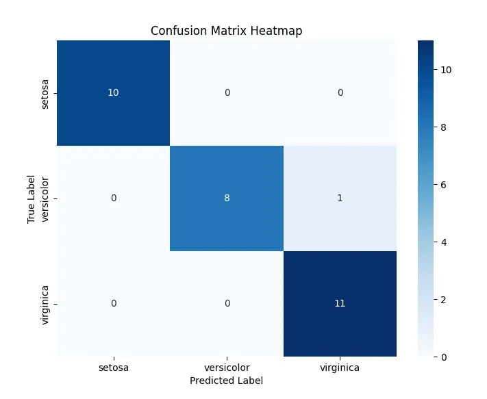
The model achieved strong performance, with only one misclassification. This emphasizes the simplicity of the Iris dataset, which allows for high accuracy even without regularization or normalization. Because we have previously demonstrated the impact of normalization and regularization in finding the optimal model performance, we omit these for this example. Instead, we focus on another crucial aspect of logistic regression—visualizing the Loss over Epochs.

Loss ver Epochs: Loss over epochs is a visual representation of how the model’s training loss decreases as the number of training epochs increases, reflecting the model’s convergence. This graph demonstrates the efficiency of gradient descent in optimizing the model weights. Monitoring loss convergence helps in determining whether the model is learning effectively or if adjustments are needed, such as changes in learning rate or the number of epochs. In our upcoming MNIST example, we will utilize this concept to evaluate and fine-tune the performance of a more complex, higher-dimensional model.

Do note that in our code so far, max_iter is the same as epochs.

To track the loss over epochs, modifications were made to the train and logistic_regression_predict functions. We introduced a losses list to store the loss value at each epoch, enabling us to plot it. These changes were added to a new module, log_reg_model_with_loss.py, to maintain compatibility with prior models.

def train(weights, x, y, learning_rate, epochs, regularization=None, reg_lambda=0.01, classification_type='binary'):
    losses = []  # List to hold the loss at each epoch
    for epoch in range(epochs):
        for i in range(len(y)):
            weights = update_weights(weights, x[i:i+1], y[i:i+1], learning_rate, regularization, reg_lambda, classification_type)

        # Calculate the loss at the end of each epoch
        y_pred = forward(weights, x, classification_type)
        if classification_type == 'binary':
            loss = log_loss(y, y_pred)
        elif classification_type == 'softmax':
            loss = cross_entropy_loss(y, y_pred)

        losses.append(loss)  # Store the loss value
        # Optionally print the loss for each epoch
        # print(f"Epoch {epoch + 1}/{epochs}, Loss: {loss:.4f}")

    return weights, losses  # Return both weights and losses


def logistic_regression_predict(X_train, y_train, X_test, max_iter=10000, learning_rate=0.05, type='binary', regularization=None, reg_lambda=0.01):
    # Weight initialization
    if type == 'binary':
        weights = initialize_weights(X_train.shape[1])
    elif type == 'softmax':
        num_classes = len(np.unique(y_train))
        weights = initialize_weights(X_train.shape[1], num_classes)

    # Train the model and get losses
    weights, losses = train(weights, X_train, y_train, learning_rate, max_iter, regularization, reg_lambda, type)

    # Make predictions on test set
    y_pred_probs = forward(weights, X_test, type)

    # Convert probabilities to class predictions
    if type == 'binary':
        y_pred = (y_pred_probs >= 0.5).astype(int)
    elif type == 'softmax':
        y_pred = np.argmax(y_pred_probs, axis=1)

    return np.array(y_pred), losses  # Return predictions and losses

The following script demonstrates the implementation of loss visualization for our logistic regression model:

from log_reg_model_with_loss import logistic_regression_predict
from sklearn.datasets import load_iris
from sklearn.model_selection import train_test_split
from sklearn.preprocessing import StandardScaler
import matplotlib.pyplot as plt

# Load the iris dataset
iris = load_iris()
X = iris.data
y = iris.target

# Create training set and test set
X_train, X_test, y_train, y_test = train_test_split(X, y, test_size=0.2, random_state=42)

# Normalize the features using StandardScaler
scaler = StandardScaler()
X_train = scaler.fit_transform(X_train)  # Fit to training data and transform
X_test = scaler.transform(X_test)        # Transform the test data

# Use our LogReg model and capture the losses
y_pred, losses = logistic_regression_predict(X_train, y_train, X_test, max_iter=1000, type='softmax')

# Plot the loss over epochs
plt.plot(losses)
plt.title('Loss Over Epochs')
plt.xlabel('Epochs')
plt.ylabel('Loss')
plt.grid()
plt.show()

Iris Loss over Epochs

Iris with Logistic Regression: Loss over Epochs

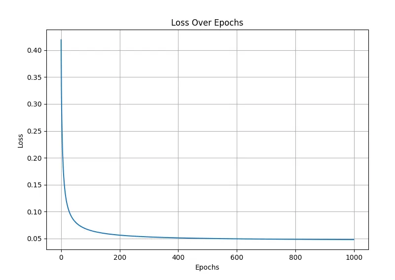
The convergence of the loss indicates that the model is learning effectively, minimizing the error in predictions with each iteration. A well-converging loss curve suggests that the gradient descent algorithm is working properly, making steady progress toward an optimal solution. This understanding is essential for our next example with the MNIST dataset.

D. MNIST (Softmax Regression)

Dataset: MNIST

The MNIST dataset is a comprehensive collection of handwritten digits that serves as a benchmark for machine learning research. It includes 60,000 training images and 10,000 testing images, each representing a grayscale digit in a 28x28-pixel format.

MNIST dataset

The MNIST Dataset - Source: deeplake

Key characteristics of the MNIST dataset:

Image size: 28x28 pixels.
Feature dimensionality: 784 (28*28).
Class labels: 10 (0-9).
Data type: Grayscale images.
Task: Multi-class classification.

By training our logistic regression model on the MNIST dataset, we’ll gain valuable insights into its ability to accurately classify handwritten digits, a fundamental challenge in computer vision and in machine learning as a whole. For this example, we will use our log_reg_model_with_loss.py module to also be able to plot the loss over epochs later on. We will also uncomment the print statement in train to be able to watch the loss over epochs in our output.

To efficiently process the data, we normalize the grayscale pixel values (ranging from 0 to 255) to be between 0 and 1, optimizing the model’s calculations. For our model, we choose max_iter=20 (to limit computational intensity) whilst the choices of learning_rate=0.05 and no regularization is purely arbitrary and personal preference.

import numpy as np
from sklearn import datasets
from sklearn.model_selection import train_test_split
from sklearn.preprocessing import StandardScaler
from sklearn.metrics import accuracy_score, precision_score, recall_score, confusion_matrix
import log_reg_model_with_loss as logr
import matplotlib.pyplot as plt
import seaborn as sns

# Load MNIST dataset from sklearn (or load_digits if MNIST is too large)
mnist = datasets.fetch_openml('mnist_784', version=1)
X, y = mnist.data, mnist.target.astype(int)

# Normalize the dataset using StandardScaler
scaler = StandardScaler()
X = scaler.fit_transform(X)

# Split the dataset into training and testing sets
X_train, X_test, y_train, y_test = train_test_split(X, y, test_size=0.2, random_state=42)

# Define the parameters for the logistic regression model
max_iter = 20
learning_rate = 0.05
regularization = None
reg_lambda = 0.0
logreg_type = 'softmax'

# Use our Logistic Regression model and capture the losses
y_pred, losses = logr.logistic_regression_predict(X_train, y_train, X_test, max_iter=max_iter, learning_rate=learning_rate,
                                                  regularization=regularization, reg_lambda=reg_lambda, type=logreg_type)

# Calculate evaluation metrics
accuracy = accuracy_score(y_test, y_pred)
precision = precision_score(y_test, y_pred, average='macro')
recall = recall_score(y_test, y_pred, average='macro')
conf_matrix = confusion_matrix(y_test, y_pred)

# Print out the evaluation metrics
print("Accuracy:", accuracy)
print("Precision (macro):", precision)
print("Recall (macro):", recall)

Epoch 1/20, Loss: 2.3067
Epoch 2/20, Loss: 2.1386
Epoch 3/20, Loss: 2.0750
Epoch 4/20, Loss: 2.0085
Epoch 5/20, Loss: 2.0617
Epoch 6/20, Loss: 1.9551
Epoch 7/20, Loss: 2.0166
Epoch 8/20, Loss: 1.9354
Epoch 9/20, Loss: 1.8955
Epoch 10/20, Loss: 1.9309
Epoch 11/20, Loss: 2.0341
Epoch 12/20, Loss: 1.9088
Epoch 13/20, Loss: 1.9094
Epoch 14/20, Loss: 1.8561
Epoch 15/20, Loss: 1.9609
Epoch 16/20, Loss: 1.8854
Epoch 17/20, Loss: 1.9777
Epoch 18/20, Loss: 1.8312
Epoch 19/20, Loss: 1.8527
Epoch 20/20, Loss: 1.9109
Accuracy: 0.8862142857142857
Precision (macro): 0.8853723951900576
Recall (macro): 0.8847057417620553

The decreasing trend in the loss value over epochs indicates effective learning, despite some fluctuation. By the final epoch, our model achieved an accuracy of approximately 88.6%, with macro-averaged precision and recall around 88.5% and 88.4%, respectively. Given the complexity of this high-dimensional dataset (784 features), these metrics indicate promising model performance. Let’s plot the loss over epochs for better visuallization:

# Plot the loss over epochs
plt.figure(figsize=(10, 6))
plt.plot(losses, label='Loss over Epochs')
plt.title('Loss Over Epochs for MNIST Dataset')
plt.xlabel('Epochs')
plt.ylabel('Loss')
plt.grid(True)
plt.legend()
plt.show()

MNIST Loss over Epochs

MNIST with Logistic Regression: Loss over Epochs

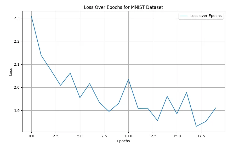
The fluctuating behavior of the loss function during training may be influenced by several factors, including the non-convex nature of the loss landscape, choice of learning rate, and possible noise in the data. This is the main reason why we choose max_iter (epochs) to be 20 as with hindsight, more epochs past that point did not result in any further decrease to the loss. Next, we look at our heatmap confusion matrix, which should be increadibly informative considering we have 10 classes to evaluate.

# Plot the confusion matrix using a heatmap
plt.figure(figsize=(10, 8))
sns.heatmap(conf_matrix, annot=True, cmap='Blues', fmt='g', cbar=True, linewidths=0.5)
plt.title('Confusion Matrix Heatmap for MNIST Dataset')
plt.xlabel('Predicted Label')
plt.ylabel('True Label')
plt.show()

MNIST Heatmap 1

MNIST with Logistic Regression: Heatmap Confusion Matrix

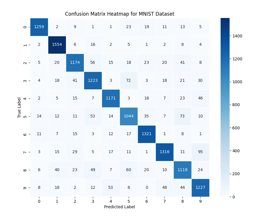
The confusion matrix demonstrates that most predictions align well with the true labels, as indicated by the dominance along the principal diagonal. To better understand the model’s misclassifications, we create a version of the confusion matrix that highlights incorrect predictions by zeroing out the diagonal elements:

# Plot the confusion matrix using a heatmap (without diagonal emphasis)
conf_matrix_no_diag = conf_matrix.copy()
np.fill_diagonal(conf_matrix_no_diag, 0)

plt.figure(figsize=(10, 8))
sns.heatmap(conf_matrix_no_diag, annot=True, cmap='Blues', fmt='g', cbar=True, linewidths=0.5)
plt.title('Confusion Matrix Heatmap for MNIST Dataset (FP & FN Emphasized)')
plt.xlabel('Predicted Label')
plt.ylabel('True Label')
plt.show()

MNIST Heatmap 2

MNIST with Logistic Regression: Heatmap Confusion Matrix - Error Emphasized

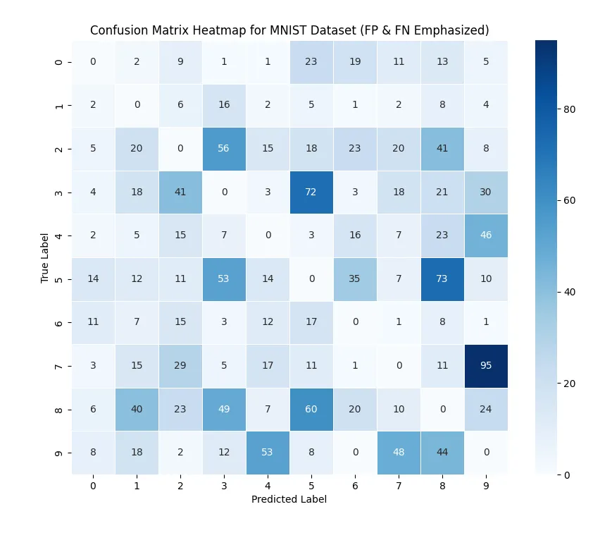
This adjusted heatmap reveals the classes where the model struggles most. For instance, it frequently confuses the digits 9 and 7, 5 and 3, and 8 and 5. This analysis helps identify specific areas for potential model improvement, such as adjusting hyperparameters or incorporating feature engineering.

In general, our implementation logistic regression performed effectively on the MNIST dataset, achieving high accuracy and demonstrating consistent learning throughout the training epochs. The observed loss reduction and detailed confusion matrix analysis validated the model’s ability to distinguish handwritten digits, highlighting both strengths and common areas of confusion.

These results mark a successful conclusion to our testing session, showcasing the potential of logistic regression for multi-class classification tasks, even in high-dimensional contexts like MNIST.

IV, Conclusion

In this post, we embarked on a comprehensive journey to implement logistic regression from scratch, starting with building a fundamental understanding of the underlying concepts and progressively enhancing the model to handle more complex tasks. We began with binary logistic regression using the sigmoid function, exploring how it effectively differentiates between two classes. Leveraging this foundation, we extended the implementation to support multi-class classification through the one-vs-rest approach and then moved on to softmax regression, which allowed us to tackle true multi-class problems more efficiently.

Throughout this process, we introduced key components like regularization to prevent overfitting, encapsulating all functionalities into a reusable module. The testing phase showcased the power and flexibility of our implementation through a series of increasingly challenging examples.

First, we used a simple binary example—study hours versus test results—to illustrate the core principle of sigmoid-based classification and its effectiveness in decision-making tasks. We then applied our model to the graduate admission dataset, performing a grid search to identify optimal regularization and lambda values, demonstrating the impact of hyperparameter tuning on performance.

With the Iris dataset, we introduced loss visualization over training epochs, illustrating how the model learns over time, and further visualized model performance with a confusion matrix heatmap. Finally, we tested our softmax regression on the MNIST dataset, successfully demonstrating the ability of our implementation to manage high-dimensional data and achieve accurate results, supported by the analysis of loss behavior and detailed error diagnostics.

In conclusion, this project not only highlighted the process of building logistic regression from the ground up but also demonstrated its application across diverse classification tasks. By breaking down each stage—binary classification, multi-class extension, and model refinement—this post provided a deep understanding of logistic regression and its versatility. With a solid foundation in these core concepts, you are now well-equipped to apply logistic regression in real-world scenarios, explore advanced optimization techniques, or venture into more sophisticated machine learning models.

Epilouge

This model is definitely one of the most complex implementations I’ve tackled from scratch so far, and this post reflects that complexity. It’s the longest one I’ve ever written, taking around three days to fully bring everything together. Throughout this journey, I realized just how foundational logistic regression is—not only as a stand-alone machine learning algorithm but also in how it connects to more advanced topics like neural networks and deep learning.

The fascinating part for me has been recognizing that, while machine learning isn’t rigidly sequential like mathematics—you don’t have to learn A before you can understand B—the connections between these concepts are often surprising and even delightful, much like an unexpected cameo in a favorite movie. It makes the entire field feel so interconnected, and every new idea learned often provides a key insight into something else, sometimes in ways I didn’t anticipate.

I’m planning to implement Principal Component Analysis (PCA), a tool that I’ve long wanted to understand better through hands-on coding. I also have some unfinished business with linear regression from scratch—an overdue project that I’m eager to complete. For now, these implementation posts are my main focus, as they give me the chance to fully engage with each concept and, most importantly, share that journey with you. Until next time.

Yuk 10/05/2024

References and Extras:

Cao Van Chung - Multinomial Logistic Regresson (Softmax Regression).
Sandro Sperandei - Understanding logistic regression analysis.
Joseph M. Hilbe - Logistic Regression.
David M. Hosmer & Stanley Lemeshow - Applied Logistic Regression.
Dhairya Kothari - MNIST with Logistic Regression.
Chriscc - Logistic Regression for MNIST with regularization.