K-NN - Python implementation from scratch
Table of Content
Block
Remarks
This blog post dives straight into implementing a K-Nearest Neighbors (KNN) model from scratch in Python. We’ll focus on the core functionalities without going into extensive explanations of the KNN algorithm itself.
While KNN is a well-known and relatively simple algorithm, in-depth theoretical explanations might be better suited for a separate post. Considering the curriculum of my current machine learning course, this implementation-focused approach seems more relevant for my current needs.
I, Overview
A. K-Nearest-Neighbor
If you’re familiar with machine learning, you probably know that KNN is a super intuitive and straightforward algorithm used for both classification and regression tasks. The idea is pretty simple: when you want to make a prediction for a new data point, KNN looks at the ‘K’ closest data points in your training set. It then bases its prediction on the majority class (for classification) or the average (for regression) of those neighbors. Think of it like asking your friends for advice—if most of them suggest the same thing, you’re likely to go with that!
B. Limitation of this Post
Before we jump into coding, let’s quickly cover a few limitations you should keep in mind:
- Will Only Test for L2 Norm: We’ll focus on the L2 norm (Euclidean distance) for measuring distances. There are other distance metrics, but for simplicity, we’re sticking with this one.
- Curse of Dimensionality: As the number of dimensions increases, the distance between points becomes less meaningful. This can mess with our KNN model, especially in high-dimensional spaces.
- Instance-Based Models and Lazy Learning: KNN is what’s called an instance-based model. It doesn’t build a general model during training; instead, it memorizes the training instances and waits until it gets new data. This means it can be slower at prediction time, especially with large datasets.
C. Necessary Imports
Throughout this post, we will assume these imports
import numpy as np  # For numerical operations and array manipulations.
import pandas as pd  # For data manipulation and analysis, especially with DataFrames.
import matplotlib.pyplot as plt  # For creating visualizations to help understand our data and results.
D. General process of K-NN
- Training: K-NN stores the training data without any explicit model fitting.
- Distance Calculation: For new, unseen data, compute the distance from the new data point to each stored data point.
- Sorting: Sort the calculated distances in ascending order while retaining their corresponding indices.
- Prediction: For classification, determine the predicted class by majority vote among the nearest neighbors; for regression, calculate the mean or median of the nearest values.
E. Final Goal of this Post
The aim of this journey is to create a flexible K-NN function that can handle both classification and regression tasks. Here’s the plan:
def k_nearest_neighbor_predict(X_train, y_train, X_test, k=3, distance_func=euclidean_distance, regression=False):
    """k-NN Prediction (Classification or Regression).

    This function predicts the output for a given test set using the k-nearest neighbors algorithm.
    It can perform either classification or regression based on the `regression` flag.

    Parameters:
        X_train: numpy.ndarray
            A 2D array of training samples (shape: [n_samples, n_features]).
        y_train: numpy.ndarray
            A 1D array of training labels or values (shape: [n_samples]).
        X_test: numpy.ndarray
            A 2D array of test samples (shape: [m_samples, n_features]).
        k: int
            Number of nearest neighbors to consider (default is 3).
        distance_func: function
            Function to calculate the distance between points (default is euclidean_distance).
        regression: bool
            If True, perform regression; otherwise, perform classification (default is False).

    Returns:
        numpy.ndarray
            A 1D array of predicted labels (for classification) or predicted values (for regression)
            for the test samples (shape: [m_samples]).
    """
    return np.array(y_pred)
So with that being said, let’s get coding.
II, Building the Model
Distance Metrics
When it comes to KNN, calculating the distance between data points is crucial, and there are several ways to do this. Here are four popular distance metrics:
Block
- Euclidean Distance (L2 Norm): This is the most commonly used distance metric. It measures the straight-line distance between two points in Euclidean space. Essentially, it’s like finding the length of the shortest path connecting two points. It’s given by the formula:
Block
- Manhattan Distance (L1 Norm): Also known as “taxicab” or “city block” distance, this metric sums the absolute differences between the coordinates of two points. Imagine navigating a grid-like city; you can only move along the streets, making it a practical way to measure distance in urban settings:
Block
- Minkowski Distance: This metric generalizes both Euclidean and Manhattan distances. It introduces a parameter that defines the order of the distance calculation. When , it becomes Euclidean distance, and when , it becomes Manhattan distance. It’s defined as:
Block
- Chebyshev Distance: This metric is based on the maximum absolute difference among the dimensions. It’s useful in certain applications, such as chess, where the distance between pieces can be measured by how far apart they are in the worst case:
Block
Below is the Python implementation for the 4 distance metrics mentioned above:
# All functions returns a single scalar value
def euclidean_distance(x1, x2): # We will only be using this
    """Calculate the Euclidean distance between two vectors."""
    return np.sqrt(np.sum((x1 - x2) ** 2))

def manhattan_distance(x1, x2):
    """Calculate the Manhattan distance between two vectors."""
    return np.sum(np.abs(x1 - x2))

def minkowski_distance(x1, x2, p=2):
    """Calculate the Minkowski distance between two vectors."""
    return np.power(np.sum(np.abs(x1 - x2) ** p), 1/p)

def chebyshev_distance(x1, x2):
    """Calculate the Chebyshev distance between two vectors."""
    return np.max(np.abs(x1 - x2))
Hamming Distance
For completeness, there’s also Hamming Distance, which measures the number of positions at which two strings of equal length differ. It’s particularly useful for categorical data and binary vectors, but we won’t cover it in this post for simplicity. Hamming Distance - Wikipedia
Distance Calculation and Majority Voting
A. Distance Calculation
To make KNN work, we need to calculate the distances between our test sample and all training samples. We’ll do this using our distance functions. The compute_distances function does exactly that, taking in our training data, a single test sample, and a chosen distance function (defaulting to Euclidean distance). It returns a list of distances between the test sample and each training sample.
def compute_distances(X_train, x_test, distance_func=euclidean_distance):
    """Compute distances between a test sample and each training sample.

    Parameters:
        X_train: numpy.ndarray
            A 2D array of training samples (shape: [n_samples, n_features]).
        x_test: numpy.ndarray
            A 1D array representing a single test sample (shape: [n_features]).
        distance_func: function
            A function to calculate the distance between two points (default is euclidean_distance).

    Returns:
        list
            A list of distances between x_test and each sample in X_train.
    """
    distances = []

    for x_train in X_train:
        # Calculate the distance between the training sample and the test sample
        distance = distance_func(x_train, x_test)
        distances.append(distance)

    return distances
B. Majority Vote
Next up, we need to determine which label (or value) to assign to our test sample based on its nearest neighbors. For classification, we use a majority voting system. The majority_vote function counts the occurrences of each label among the nearest neighbors and returns the label that appears most frequently. Here’s how that’s implemented:
def majority_vote(labels):
    """Manually compute the majority vote from the given labels.

    Parameters:
        labels: numpy.ndarray or list
            A 1D array (or list) of labels corresponding to the nearest neighbors.

    Returns:
        scalar
            The label that appears most frequently among the input labels.
    """
    label_count = {}

    # Count occurrences of each label
    for label in labels:
        if label in label_count:
            label_count[label] += 1
        else:
            label_count[label] = 1

    # Find the label with the maximum count
    max_count = -1
    majority_label = None
    for label, count in label_count.items():
        if count > max_count:
            max_count = count
            majority_label = label

    return majority_label
K-NN for Classification
Now that we can calculate distances and determine the nearest neighbors, let’s put it all together for classification.
The k_nearest_neighbor_classification function takes our training data, labels, test samples, and the number of neighbors to consider. It uses our distance calculation and majority voting functions to predict labels for the test samples:
def k_nearest_neighbor_classification(X_train, y_train, X_test, k=3, distance_func=euclidean_distance):
    """k-NN Classification.

    Parameters:
        X_train: numpy.ndarray
            A 2D array of training samples (shape: [n_samples, n_features]).
        y_train: numpy.ndarray
            A 1D array of training labels (shape: [n_samples]).
        X_test: numpy.ndarray
            A 2D array of test samples (shape: [m_samples, n_features]).
        k: int
            Number of nearest neighbors to consider (default is 3).
        distance_func: function
            Function to calculate the distance between points (default is euclidean_distance).

    Returns:
        numpy.ndarray
            A 1D array of predicted labels for the test samples (shape: [m_samples]).
    """
    y_pred = []

    for x_test in X_test:
        # Compute distances from the test sample to all training samples
        dists = compute_distances(X_train, x_test, distance_func)

        # Create a dictionary of indices and distances
        distance_dict = {idx: dist for idx, dist in enumerate(dists)}

        # Sort the dictionary by distances and get the nearest k indices
        sorted_distance_dict = dict(sorted(distance_dict.items(), key=lambda item: item[1]))
        nearest_indices = list(sorted_distance_dict.keys())[:k]

        # Get the corresponding labels from y_train
        nearest_labels = y_train[np.array(nearest_indices)]

        # Predict the label by majority vote among the nearest labels
        pred = majority_vote(nearest_labels)

        y_pred.append(pred)

    return np.array(y_pred)
K-NN for Regression
Now, if you’re working with regression, we can adapt the process slightly. Instead of majority voting, we’ll take the average of the nearest neighbors’ values.
The k_nearest_neighbor_regression function is similar to the classification one, but it calculates the mean (note that you can also use median in some cases) of the nearest values instead of a label:
def k_nearest_neighbor_regression(X_train, y_train, X_test, k=3, distance_func=euclidean_distance):
    """k-NN Regression.

    Parameters:
        X_train: numpy.ndarray
            A 2D array of training samples (shape: [n_samples, n_features]).
        y_train: numpy.ndarray
            A 1D array of training values (shape: [n_samples]).
        X_test: numpy.ndarray
            A 2D array of test samples (shape: [m_samples, n_features]).
        k: int
            Number of nearest neighbors to consider (default is 3).
        distance_func: function
            Function to calculate the distance between points (default is euclidean_distance).

    Returns:
        numpy.ndarray
            A 1D array of predicted values for the test samples (shape: [m_samples]).
    """
    y_pred = []

    for x_test in X_test:
        # Compute distances from the test sample to all training samples
        dists = compute_distances(X_train, x_test, distance_func)

        # Create a dictionary of indices and distances
        distance_dict = {idx: dist for idx, dist in enumerate(dists)}

        # Sort the dictionary by distances and get the nearest k indices
        sorted_distance_dict = dict(sorted(distance_dict.items(), key=lambda item: item[1]))
        nearest_indices = list(sorted_distance_dict.keys())[:k]

        # Get the corresponding values from y_train
        nearest_values = y_train[np.array(nearest_indices)]

        # Calculate the mean of the nearest values to make the prediction
        pred = np.mean(nearest_values)
        y_pred.append(pred)

    return np.array(y_pred)
Final result
To simplify usage, we’ll create a unified function that can handle both classification and regression tasks.
The k_nearest_neighbor_predict function checks the regression flag and performs the appropriate operation accordingly:
def k_nearest_neighbor_predict(X_train, y_train, X_test, k=3, distance_func=euclidean_distance, regression=False):
    """k-NN Prediction (Classification or Regression).

    This function predicts the output for a given test set using the k-nearest neighbors algorithm.
    It can perform either classification or regression based on the `regression` flag.

    Parameters:
        X_train: numpy.ndarray
            A 2D array of training samples (shape: [n_samples, n_features]).
        y_train: numpy.ndarray
            A 1D array of training labels or values (shape: [n_samples]).
        X_test: numpy.ndarray
            A 2D array of test samples (shape: [m_samples, n_features]).
        k: int
            Number of nearest neighbors to consider (default is 3).
        distance_func: function
            Function to calculate the distance between points (default is euclidean_distance).
        regression: bool
            If True, perform regression; otherwise, perform classification (default is False).

    Returns:
        numpy.ndarray
            A 1D array of predicted labels (for classification) or predicted values (for regression)
            for the test samples (shape: [m_samples]).
    """
    y_pred = []

    for x_test in X_test:
        # Compute distances from the test sample to all training samples
        dists = compute_distances(X_train, x_test, distance_func)

        # Create a dictionary of indices and distances
        distance_dict = {idx: dist for idx, dist in enumerate(dists)}

        # Sort the dictionary by distances and get the nearest k indices
        sorted_distance_dict = dict(sorted(distance_dict.items(), key=lambda item: item[1]))
        nearest_indices = list(sorted_distance_dict.keys())[:k]

        # Get the corresponding labels or values from y_train
        nearest_values = y_train[np.array(nearest_indices)]

        if regression:
            # If performing regression, calculate the mean of the nearest values
            pred = np.mean(nearest_values)
        else:
            # If performing classification, predict the label by majority vote
            pred = majority_vote(nearest_values)

        y_pred.append(pred)

    return np.array(y_pred)
With all these components in place, you now have a complete K-NN model that can classify and regress based on the nearest neighbors in your dataset! In the next section, we’ll explore how to evaluate the performance of our K-NN model.
III, Testing the Model
For ease of use and comprehensiveness, let’s encapsulates our model into knn_model.py:
import numpy as np

def euclidean_distance(x1, x2):
    return np.sqrt(np.sum((x1 - x2) ** 2))

def manhattan_distance(x1, x2):
    return np.sum(np.abs(x1 - x2))

def minkowski_distance(x1, x2, p=2):
    return np.power(np.sum(np.abs(x1 - x2) ** p), 1/p)

def chebyshev_distance(x1, x2):
    return np.max(np.abs(x1 - x2))

def compute_distances(X_train, x_test, distance_func=euclidean_distance):
    distances = []

    for x_train in X_train:
        distance = distance_func(x_train, x_test)
        distances.append(distance)

    return distances

def majority_vote(labels):
    label_count = {}

    for label in labels:
        if label in label_count:
            label_count[label] += 1
        else:
            label_count[label] = 1

    max_count = -1
    majority_label = None
    for label, count in label_count.items():
        if count > max_count:
            max_count = count
            majority_label = label

    return majority_label


def k_nearest_neighbor_predict(X_train, y_train, X_test, k=3, regression=False, distance_func=euclidean_distance):
    y_pred = []

    for x_test in X_test:
        dists = compute_distances(X_train, x_test, distance_func)
        distance_dict = {idx: dist for idx, dist in enumerate(dists)}
        sorted_distance_dict = dict(sorted(distance_dict.items(), key=lambda item: item[1]))
        nearest_indices = list(sorted_distance_dict.keys())[:k]
        nearest_values = y_train[np.array(nearest_indices)]

        if regression:
            pred = np.mean(nearest_values)
        else:
            pred = majority_vote(nearest_values)

        y_pred.append(pred)

    return np.array(y_pred)
Evaluation Metrics for K-NN
A. Classification Evaluation Metrics
-
Accuracy: Measures the proportion of correctly predicted instances among the total instances. It’s a straightforward metric but can be misleading in imbalanced datasets.
-
Precision: Indicates the proportion of predicted positive instances that are actually positive, making it important in situations where false positives are costly.
-
Recall (Sensitivity): Measures the proportion of actual positive instances that were correctly predicted. It’s crucial when missing a positive instance is costly.
-
Confusion Matrix: A summary that shows the counts of true positives, true negatives, false positives, and false negatives, helping to visualize the model’s performance.
B. Regression Evaluation Metrics
-
Mean Squared Error (MSE): Quantifies the average squared difference between predicted and actual values, with lower values indicating better model performance.
-
R-Squared (): Represents the proportion of variance in the dependent variable explained by the independent variables. Higher values indicate a better fit for the model.
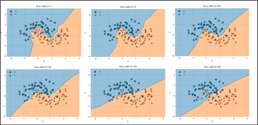
C. Decision Boundary
A decision boundary is a hypersurface that separates different classes in a classification task. In the context of K-NN, it represents the regions in the feature space where the algorithm predicts one class over another. As K-NN uses the majority class of the nearest neighbors to make predictions, the decision boundary can be complex and non-linear, adapting to the distribution of the training data. Visualizing decision boundaries helps in understanding how well the model can differentiate between classes in various regions of the feature space. In this post we will not be going deep into this concept but keep in mind that most K-NN models are visualized by Decision Boundary.
Examples
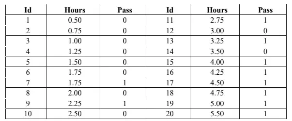
A. Study Hours (Binary Classification)
In this example, we utilize a dataset that captures the relationship between study hours and the outcome of passing a test, represented in the column ‘Pass’ (0 for Passed and 1 for Not Passed). This dataset serves as a classic case for binary classification, where we aim to predict whether a student will pass based on the number of hours studied.
import numpy as np
import knn_model as knn # Assume we have put all of our function into knn_model.py
from sklearn.model_selection import train_test_split
from sklearn.metrics import accuracy_score, precision_score, recall_score, confusion_matrix

# Initiating data
hours = np.array([0.50, 0.75, 1.00, 1.25, 1.50, 1.75, 1.75, 2.00, 2.25, 2.50,
                  2.75, 3.00, 3.25, 3.50, 4.00, 4.25, 4.50, 4.75, 5.00, 5.50])
pass_array = np.array([0, 0, 0, 0, 0, 0, 1, 0, 0, 0,
                       1, 0, 1, 0, 1, 1, 1, 1, 1, 1])

# Create training set and test set, because 'Hours' is sorted ascending, we need to shuffle the data
X_train, X_test, y_train, y_test = train_test_split(hours, pass_array, train_size=15, test_size=5, random_state=42)

# Use our K-NN Model
y_pred = knn.k_nearest_neighbor_predict(X_train, y_train, X_test, k=3)

# Print out evaluation metrics
accuracy = accuracy_score(y_test, y_pred)
print("Accuracy:", accuracy)
precision = precision_score(y_test, y_pred)
print("Precision:", precision)
recall = recall_score(y_test, y_pred)
print("Recall:", recall)
conf_matrix = confusion_matrix(y_test, y_pred)
print("Confusion Matrix:\n", conf_matrix)
By applying our K-NN model with K = 3, we can classify test samples based on their nearest neighbors in the training set. The evaluation metrics—accuracy, precision, and recall—indicate that our model performs perfectly, achieving an accuracy of 1.0. The confusion matrix further confirms this, showing that all predictions were correct: three students passed, and two did not.
Accuracy: 1.0
Precision: 1.0
Recall: 1.0
Confusion Matrix:
 [[3 0]
 [0 2]]
Overall, this result suggests that the relationship between study hours and test outcomes is quite clear, allowing the K-NN model to effectively distinguish between the two classes.
B. Iris (Multi-class Classification)
In the Iris dataset example, we extend our K-NN model to handle multi-class classification, where we classify different species of iris flowers based on various features. This dataset is widely used in machine learning as a benchmark due to its simplicity and well-defined classes.
import knn_model as knn
from sklearn.datasets import load_iris
from sklearn.model_selection import train_test_split
from sklearn.metrics import accuracy_score, precision_score, recall_score, confusion_matrix

# Load the iris dataset
iris = load_iris()
X = iris.data
y = iris.target

# Create training set and test set
X_train, X_test, y_train, y_test = train_test_split(X, y, test_size=0.2, random_state=42)

# Use our K-NN Model
y_pred = knn.k_nearest_neighbor_predict(X_train, y_train, X_test, k=3)

# Print out evaluation metrics for multiclass
accuracy = accuracy_score(y_test, y_pred)
print("Accuracy:", accuracy)

# For multiclass problems, specify the average type for precision and recall
precision = precision_score(y_test, y_pred, average='macro')
print("Precision (macro):", precision)

recall = recall_score(y_test, y_pred, average='macro')
print("Recall (macro):", recall)

# Compute and display the confusion matrix
conf_matrix = confusion_matrix(y_test, y_pred)
print("Confusion Matrix:\n", conf_matrix)
After splitting the data into training and test sets, we apply our K-NN model with K = 3. The evaluation metrics again reveal perfect performance, with an accuracy of 1.0. The precision and recall values, computed using the macro average, further confirm the model’s effectiveness across all classes. The confusion matrix indicates that all species were correctly classified, with no misclassifications.
Accuracy: 1.0
Precision (macro): 1.0
Recall (macro): 1.0
Confusion Matrix:
 [[10  0  0]
 [ 0  9  0]
 [ 0  0 11]]
This demonstrates the robustness of the K-NN model in handling multi-class scenarios, showcasing its ability to identify and differentiate between the distinct classes present in the dataset.
C. Temp vs. Pressure (Single Regression)
In this example, we explore the relationship between temperature and pressure using both K-NN and linear regression techniques. The dataset consists of temperature readings and their corresponding pressure values.
import numpy as np
import knn_model as knn
import matplotlib.pyplot as plt
from sklearn.metrics import mean_squared_error, r2_score
from sklearn.linear_model import LinearRegression

# Initiating data
temp = np.array([194.5, 194.3, 197.9, 198.4, 199.4, 199.9, 200.9, 201.1, 201.4, 201.3,
                 203.6, 204.6, 209.5, 208.6, 210.7, 211.9, 212.2])
pressure = np.array([20.79, 20.79, 22.4, 22.67, 23.15, 23.35, 23.89, 23.99, 24.02, 24.01,
                     25.14, 26.57, 28.49, 27.76, 29.04, 29.88, 30.06])

# Create training set and test set (no shuffling)
X_train = temp[:14].reshape(-1, 1)
y_train = pressure[:14]
X_test = temp[14:].reshape(-1, 1)
y_test = pressure[14:]

# Use our K-NN Model for Regression
y_pred_knn = knn.k_nearest_neighbor_predict(X_train.flatten(), y_train, X_test.flatten(), k=3, regression=True)

# Print the evaluation metrics for K-NN
mse_knn = mean_squared_error(y_test, y_pred_knn)
r2_knn = r2_score(y_test, y_pred_knn)
print("K-NN Mean Squared Error (MSE):", mse_knn)
print("K-NN R-squared (R²):", r2_knn)

# Fit sk-learn's Linear Regression Model
lin_reg = LinearRegression()
lin_reg.fit(X_train, y_train)

# Create predictions for the entire temperature range (for plotting the line)
X_all = np.linspace(temp.min(), temp.max(), 100).reshape(-1, 1)
y_pred_all_lr = lin_reg.predict(X_all)

# Create predictions for the test set
y_pred_lr = lin_reg.predict(X_test)

# Print the evaluation metrics for Linear Regression
mse_lr = mean_squared_error(y_test, y_pred_lr)
r2_lr = r2_score(y_test, y_pred_lr)
print("Linear Regression Mean Squared Error (MSE):", mse_lr)
print("Linear Regression R-squared (R²):", r2_lr)

# Visualization: Side-by-side plots for K-NN and Linear Regression
fig, axs = plt.subplots(1, 2, figsize=(18, 6))

# K-NN Plot
axs[0].scatter(X_train, y_train, color='blue', label='Training Data', alpha=0.6)
axs[0].scatter(X_test, y_test, color='green', label='Test Data', alpha=0.6)
axs[0].scatter(X_test, y_pred_knn, color='red', label='K-NN Predicted Values', marker='x', s=100)
axs[0].set_xlabel('Temperature')
axs[0].set_ylabel('Pressure')
axs[0].set_title('K-NN Regression: Temperature vs Pressure (Actual vs Predicted)')
axs[0].legend()
axs[0].grid(True)

# Linear Regression Plot
axs[1].scatter(X_train, y_train, color='blue', label='Training Data', alpha=0.6)
axs[1].scatter(X_test, y_test, color='green', label='Test Data', alpha=0.6)
axs[1].plot(X_all, y_pred_all_lr, color='red', linestyle='--', label='Linear Regression Predicted Line', linewidth=2)
axs[1].scatter(X_test, y_pred_lr, color='red', marker='x', s=100)  # Mark test predictions
axs[1].set_xlabel('Temperature')
axs[1].set_ylabel('Pressure')
axs[1].set_title('Linear Regression: Temperature vs Pressure (Actual vs Predicted)')
axs[1].legend()
axs[1].grid(True)

plt.show()
The K-NN model, configured with K = 3, demonstrated limitations in its predictive capabilities. Its Mean Squared Error (MSE) was relatively high at 4.41, and the R-squared value was notably low at -21.34. This indicates that the model struggled to generalize well, particularly when making predictions outside the range of the training data. As seen in the plots, K-NN predictions failed to extend beyond the training set, resulting in poor performance for extrapolated values.
In contrast, the linear regression model excelled in this scenario, achieving a much lower MSE of 0.06 and a positive R-squared value of 0.72. The linear regression line effectively captures the underlying trend in the data, allowing for better predictions both within and beyond the training range. This highlights the model’s strength in establishing a continuous relationship between the variables.
K-NN Mean Squared Error (MSE): 4.413777777777778
K-NN R-squared (R²): -21.336932073774197

Linear Regression Mean Squared Error (MSE): 0.05586233584990541
Linear Regression R-squared (R²): 0.717295871204932
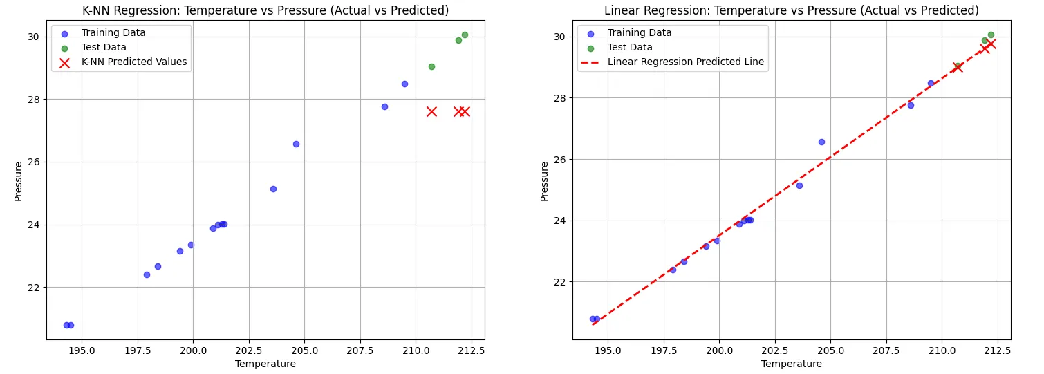
The side-by-side visualization clearly illustrates these differences, with the K-NN model’s predictions marked by discrete points that do not extend beyond the training data, while linear regression provides a smooth and consistent predictive line. Overall, this comparison underscores the limitations of K-NN in regression tasks, especially in situations where extrapolation is necessary, while demonstrating the advantages of linear regression in capturing trends and making robust predictions.
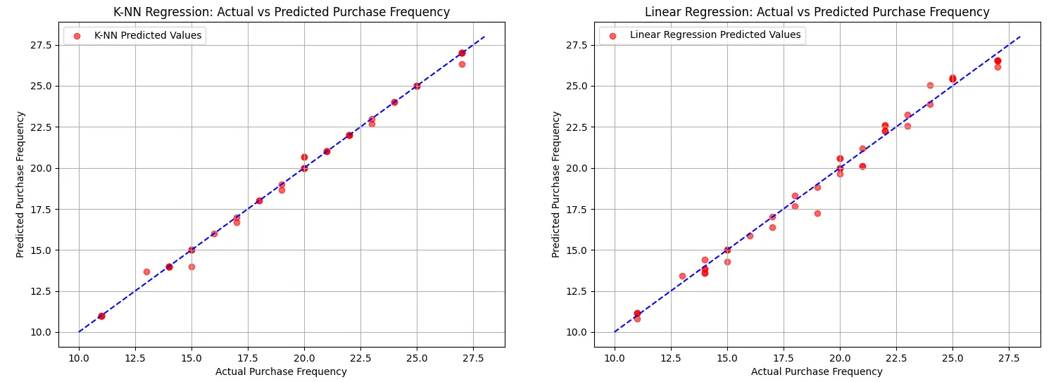
D. Customer Purchasing Behavior (Multiple Regression)
In this analysis, we examine customer purchasing behavior using both K-NN and linear regression models to predict purchase frequency based on various features. The dataset was cleaned by removing unnecessary columns, ensuring that the features were relevant for predicting the target variable.
import numpy as np
import pandas as pd
import knn_model as knn
import matplotlib.pyplot as plt
from sklearn.metrics import mean_squared_error, r2_score
from sklearn.linear_model import LinearRegression
from sklearn.model_selection import train_test_split

# Load the data
data = pd.read_csv('Customer Purchasing Behaviors.csv')

# Drop unnecessary columns
data = data.drop(columns=['user_id', 'region'])

# Define features (X) and target (y)
X = data.drop(columns=['purchase_frequency']).values  # All columns except 'purchase_frequency'
y = data['purchase_frequency'].values  # Target variable

# Convert everything to float
X = X.astype(float)
y = y.astype(float)

# Split the data into training and testing sets
X_train, X_test, y_train, y_test = train_test_split(X, y, test_size=0.2, random_state=42)

# Use our K-NN Model for Regression
y_pred_knn = knn.k_nearest_neighbor_predict(X_train, y_train, X_test, k=3, regression=True)

# Print the evaluation metrics for K-NN
mse_knn = mean_squared_error(y_test, y_pred_knn)
r2_knn = r2_score(y_test, y_pred_knn)
print("K-NN Mean Squared Error (MSE):", mse_knn)
print("K-NN R-squared (R²):", r2_knn)

# Fit sk-learn's Linear Regression Model
lin_reg = LinearRegression()
lin_reg.fit(X_train, y_train)

# Create predictions for the test set
y_pred_lr = lin_reg.predict(X_test)

# Print the evaluation metrics for Linear Regression
mse_lr = mean_squared_error(y_test, y_pred_lr)
r2_lr = r2_score(y_test, y_pred_lr)
print("Linear Regression Mean Squared Error (MSE):", mse_lr)
print("Linear Regression R-squared (R²):", r2_lr)

# Visualization: Side-by-side plots for K-NN and Linear Regression
fig, axs = plt.subplots(1, 2, figsize=(18, 6))

# K-NN Plot (Scatter plot for predictions)
axs[0].scatter(y_test, y_pred_knn, color='red', label='K-NN Predicted Values', alpha=0.6)
axs[0].set_xlabel('Actual Purchase Frequency')
axs[0].set_ylabel('Predicted Purchase Frequency')
axs[0].set_title('K-NN Regression: Actual vs Predicted Purchase Frequency')
axs[0].plot([y.min(), y.max()], [y.min(), y.max()], color='blue', linestyle='--')  # Line of equality
axs[0].legend()
axs[0].grid(True)

# Linear Regression Plot
axs[1].scatter(y_test, y_pred_lr, color='red', label='Linear Regression Predicted Values', alpha=0.6)
axs[1].set_xlabel('Actual Purchase Frequency')
axs[1].set_ylabel('Predicted Purchase Frequency')
axs[1].set_title('Linear Regression: Actual vs Predicted Purchase Frequency')
axs[1].plot([y.min(), y.max()], [y.min(), y.max()], color='blue', linestyle='--')  # Line of equality
axs[1].legend()
axs[1].grid(True)

plt.show()
Interestingly, the K-NN model performed exceptionally well, achieving a Mean Squared Error (MSE) of 0.06 and an R-squared value of 0.997. This indicates that K-NN was able to capture the relationship between the features and the purchase frequency almost perfectly, even surpassing the linear regression model in terms of accuracy. The linear regression model, while still effective, had a higher MSE of 0.25 and an R-squared value of 0.989, demonstrating solid performance but not quite matching K-NN’s accuracy.
K-NN Mean Squared Error (MSE): 0.06481481481481485
K-NN R-squared (R²): 0.9972321075523922

Linear Regression Mean Squared Error (MSE): 0.2514097706093957
Linear Regression R-squared (R²): 0.9892636396892784
The side-by-side visualizations further highlight the performance of both models. While both models aligned closely with the line of equality (the line where predicted values equal actual values), K-NN’s predictions are notably more clustered around this line, suggesting its higher accuracy in predicting customer purchasing frequency.
Overall, this example underscores the importance of data preparation and feature selection in modeling, while also showcasing K-NN’s potential in multiple regression scenarios, even in the presence of complex relationships within high-dimensional data.
IV, Conclusion
In this post, we embarked on a hands-on journey to implement the K-Nearest Neighbors (K-NN) algorithm from scratch in Python, focusing on its core functionalities for both classification and regression tasks. We started with an overview of K-NN, highlighting its intuitive nature as a distance-based algorithm that makes predictions based on the ‘K’ closest training samples.
Throughout the implementation, we covered key aspects such as distance metrics, including Euclidean, Manhattan, Minkowski, and Chebyshev distances, which form the backbone of how K-NN operates. By developing functions for distance calculation and majority voting, we laid the groundwork for the K-NN model, allowing it to adapt flexibly to different prediction tasks.
The distinction between classification and regression was emphasized, showcasing how K-NN can efficiently handle both scenarios with minor adjustments to the prediction mechanism. Our final unified function simplified the usage of the K-NN model, making it versatile for various datasets and problem domains.
We also explored evaluation metrics to assess model performance. Through practical examples, such as the study hours dataset for binary classification and the Iris dataset for multi-class classification, we demonstrated K-NN’s ability to achieve high accuracy and reliable predictions. The comparative analysis of K-NN with linear regression in regression tasks illustrated the strengths and limitations of each approach, especially regarding extrapolation capabilities and capturing trends.
In conclusion, this comprehensive implementation not only deepens your understanding of K-NN as a powerful yet straightforward machine learning algorithm but also equips you with the tools necessary to apply K-NN effectively in real-world scenarios. As you continue to explore machine learning, consider experimenting with different datasets and tuning parameters like ‘K’ and distance metrics to observe how they influence model performance. The practical experience gained from this post serves as a solid foundation for further exploration of more complex algorithms and concepts in the field of machine learning.
References and Extras:
- V. B. Surya Prasath, Haneen Arafat Abu Alfeilat, Ahmad B. A. Hassanat, Omar Lasassmeh, Ahmad S. Tarawneh, Mahmoud Bashir Alhasanat, Hamzeh S. Eyal Salman - Effects of Distance Measure Choice on KNN Classifier Performance - A Review
- Aditya Raj - Distance Measures for Machine Learning
- Cao Van Chung - K-NN & Multinomial Logisitc Regression
- “Why do you need to scale data in KNN”
- “Thumbnail: neptune.ai”