Theoretical Advancements in Sampling-Based Motion: Planning An Analysis of RRT, RRT*, Informed RRT*, and BIT*
Table of Content
Block
Abstract
This report examines the theoretical evolution and algorithmic design of sampling-based motion planning methods, focusing on the progression from basic path feasibility to heuristically guided optimal search in continuous state spaces. Traditional discrete graph-search algorithms suffer from exponential scaling of time and space complexity in high dimensions, known as the curse of dimensionality. To address this, randomized sampling approaches are utilized. The foundational Rapidly-exploring Random Tree (RRT) algorithm provides probabilistic completeness but lacks formal guarantees of optimality. To achieve optimal solutions, RRT* introduces a rewiring mechanism based on Random Geometric Graphs (RGGs) that guarantees almost-sure asymptotic optimality. To mitigate the computational inefficiency of the uniform global sampling inherent in RRT, Informed RRT utilizes direct sampling of a prolate hyperspheroid to restrict the search strictly to the subset of states capable of improving the current path. Finally, Batch Informed Trees (BIT) unifies continuous sampling-based planning with discrete graph-search techniques by processing implicit RGGs in batches using an ordered, heuristically guided search akin to Lifelong Planning A (LPA*). This report details the core mechanisms, algorithmic design, theoretical proofs of optimality, and empirical evaluations for these four algorithms to demonstrate their efficacy in complex, high-dimensional motion planning tasks.
1. Introduction
1.1 Problem Definition
The optimal motion planning problem is formally defined within a continuous state space, denoted as $X \subseteq \mathbb{R}^n$. The subset of this state space that is in collision with obstacles is defined as the obstacle region, $X_{obs} \subset X$. The remaining obstacle-free space, in which a robot is permitted to operate, is defined as $X_{free} = X \setminus X_{obs}$ [2].
A path planning problem is specified by an initial state, $x_{start} \in X_{free}$, and a goal region, $X_{goal} \subset X_{free}$ (or a specific goal state $x_{goal}$). A path is defined as a continuous sequence of states $\sigma: \rightarrow X$, and the set of all non-trivial paths is denoted by $\Sigma$. A path is considered feasible if it is collision-free (i.e., $\sigma(\tau) \in X_{free}$ for all $\tau \in [0,1]$), begins at the initial state ($\sigma(0) = x_{start}$), and ends in the goal region ($\sigma(1) \in X_{goal}$) [2].
The objective of optimal path planning is to find a feasible path that minimizes a specific monotonic and bounded cost function, $c: \Sigma \rightarrow \mathbb{R}_{\ge 0}$ [2]. The optimal solution, denoted as $\sigma^{*}$, is mathematically defined as:
Block
The cost of this optimal path represents the theoretical minimum cost, denoted as $c_{min}$. In the context of anytime and incremental search algorithms, the cost of the best valid solution found by the algorithm at a given iteration is denoted as $c_{best}$ [3].
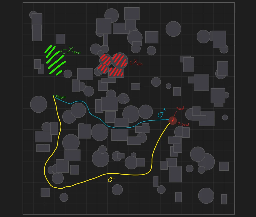
Figure 1: Path Planning Problem Visualization. A 2D configuration space showing $X_{free}, X_{obs}, x_{start}, X_{goal}$, a feasible path $\sigma$, and the optimal path $\sigma^{*}$ with cost $c_{min}$. Generated via RRT Playground [7].
1.2 The Curse of Dimensionality
The motion planning problem is commonly approached by discretizing the continuous state space and applying exact discrete graph-search methods, such as Dijkstra’s algorithm or A*. These techniques use dynamic programming to exactly solve the discrete approximation of the problem. They provide resolution completeness and resolution optimality, guaranteeing that the optimal solution will be found up to the chosen resolution of the grid.
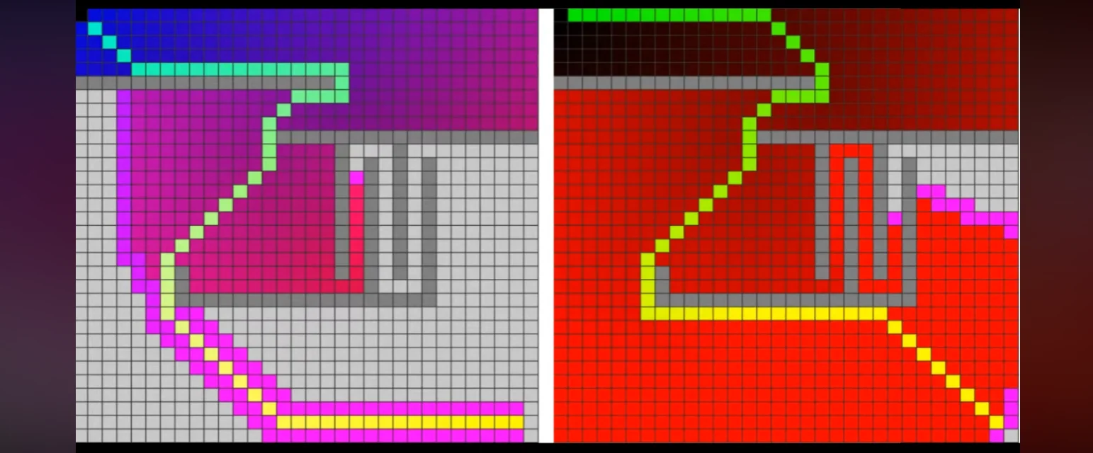
Figure 2: Discrete Graph Search. A* algorithm (left) and Dijkstra’s algorithm (right) pathfinding on a 2D grid configuration [6].
However, these discrete methods rely on an explicit representation of the configuration space and its corresponding obstacles. The quality of the resulting continuous solution is heavily dependent on the discretization; finer grids yield higher quality paths but require proportionally greater computational effort [4]. To quantify this mathematically, consider a continuous state space of dimension $d$ that is discretized into a uniform grid with $k$ discrete intervals per dimension. This discretization produces a graph consisting of $ \mid V \mid = k^d$ total vertices. Exact discrete search methods, assuming their standard baseline characteristics, must maintain an explicit representation of the problem, such as tracking visited and unvisited states in memory. This results in a worst-case space complexity of $O( \mid V \mid ) = O(k^d)$. Similarly, the worst-case time complexity to compute the shortest path on a given graph using dynamic programming is bounded by $O( \mid V \mid \log \mid V \mid + \mid E \mid )$. Substituting the number of discrete grid vertices into this bound yields a time complexity of $O(k^d \log(k^d) + \mid E \mid )$. In high-dimensional spaces, such as those required for multi-joint manipulation planning, both the memory requirements and the worst-case running time grow exponentially with respect to the number of dimensions $d$. This exponential explosion in time and space complexity is referred to as the “curse of dimensionality” [4].
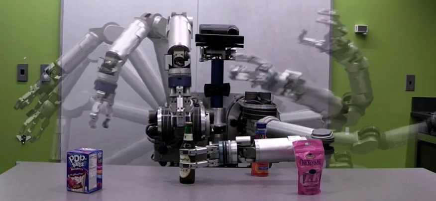
Figure 3: High-Dimensional Manipulation. The 14-DOF HERB robot manipulator navigating complex state spaces [4].
Due to this phenomenon, basic versions of the exact motion planning problem, such as the generalized piano movers problem [5], are mathematically proven to be PSPACE-hard [2]. In computational complexity theory, a PSPACE-hard classification indicates that a problem requires an amount of memory space bounded by a polynomial function of the input size, and it is at least as difficult as every other problem in the PSPACE complexity class. Because problems in this class generally require exponential execution time, the computational burden renders traditional, exact graph-search algorithms largely unsuitable for practical, high-dimensional continuous problem domains, necessitating alternative approximations and sampling methodologies [2].
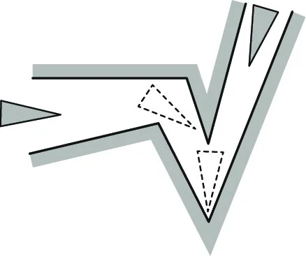
Figure 4: Piano Movers Problem. Visualization of complex continuous routing environments illustrating the challenges of exact space representation [5].
1.3 The Sampling-Based Heuristic Approach
To overcome the computational intractability associated with explicitly representing high-dimensional configuration spaces, sampling-based algorithms employ randomized approximations. Instead of constructing exact geometric boundaries for the obstacle region $X_{obs}$, these methods rely on an independent collision-checking module to evaluate the feasibility of candidate states and trajectories [2]. By randomly drawing a set of points from the continuous obstacle-free space $X_{free}$ and attempting to connect them via a local steering function, these algorithms iteratively build a graph or a tree of feasible paths.
This randomized approach provides significant computational savings, allowing planners to scale effectively into high-dimensional domains. However, bypassing the explicit discretization of the state space requires relaxing the strict completeness guarantees found in traditional discrete algorithms. While exact discrete planners are guaranteed to report failure in finite time if no solution exists, sampling-based methods generally cannot detect the absence of a path and will run indefinitely.
Consequently, sampling-based algorithms instead provide probabilistic completeness [2]. An algorithm is probabilistically complete if, for any robustly feasible path planning problem $(X_{free}, x_{init}, X_{goal})$, the probability of finding a solution approaches one as the number of iterations or samples approaches infinity. Mathematically, if $V_n$ denotes the set of vertices in the graph returned by the algorithm after $n$ iterations, the algorithm is probabilistically complete if:
Block
For robustly feasible problems, the probability that a probabilistically complete sampling-based algorithm fails to find a solution decays to zero exponentially as the number of samples increases [2]. This foundational property ensures that sampling-based heuristics will discover a feasible path rapidly, forming the basis for the specific tree- and graph-building algorithms analyzed in the subsequent sections.
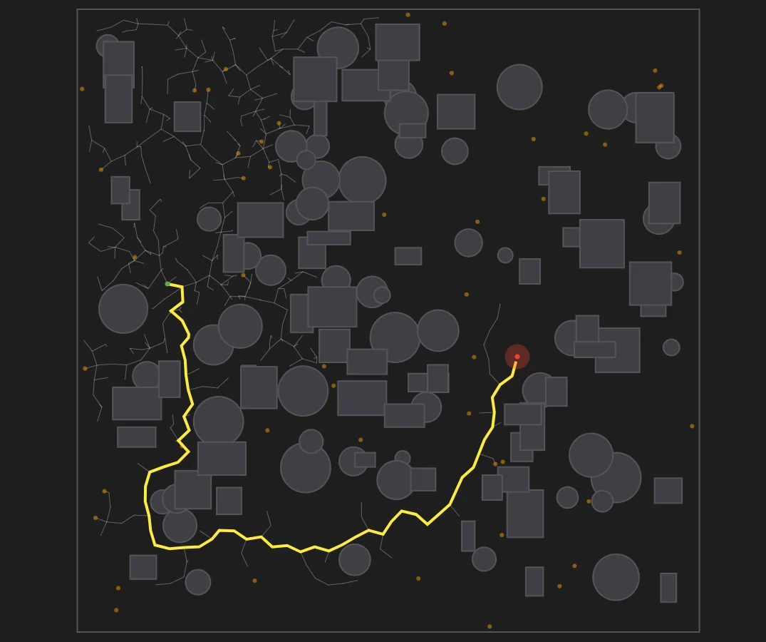
Figure 5: The Sampling-Based Heuristic Approach. The visual shows a continuous 2D space with a complex obstacle, overlaid with a set of randomly distributed sample points in the free space connected by straight line segments, demonstrating how a feasible path from start to goal is found without gridding the entire space. Generated via RRT Playground [7].
2. Methodology
The methodology of sampling-based optimal motion planning has evolved significantly to address the trade-off between computational efficiency and path optimality in high-dimensional continuous spaces. The progression analyzed in this report begins with the Rapidly-exploring Random Tree (RRT) algorithm [1], which establishes a baseline by rapidly discovering feasible paths, though it lacks formal mathematical guarantees of optimality. To address this limitation, Optimal RRT (RRT) [2] introduces a localized rewiring mechanism based on the theory of Random Geometric Graphs (RGGs) to achieve asymptotic optimality. Informed RRT [3] subsequently improves the convergence rate of RRT* by restricting the sampling domain strictly to an informed ellipsoidal subset once an initial path is found. Finally, the Batch Informed Trees (BIT*) [4] algorithm unifies this continuous sampling approach with discrete, ordered graph-search principles by processing batches of samples as implicit RGGs guided by heuristic cost estimates.
2.1 Baseline Algorithm: Rapidly-exploring Random Trees (RRT)
2.1.1 Algorithm Overview and Pseudocode
The Rapidly-exploring Random Tree (RRT) algorithm is a randomized, single-query planning method designed to rapidly explore a continuous state space without requiring an explicit grid discretization [1]. The algorithm incrementally builds a directed tree of feasible trajectories rooted at the initial condition, $x_{start}$. The fundamental logic of the algorithm is defined by the following sequence of operations:
GENERATE_RRT(x_init, K, Δt)
1  T.init(x_init);
2  for k = 1 to K do
3      x_rand ← RANDOM_STATE();
4      x_near ← NEAREST_NEIGHBOR(x_rand, T);
5      u ← SELECT_INPUT(x_rand, x_near);
6      x_new ← NEW_STATE(x_near, u, Δt);
7      T.add_vertex(x_new);
8      T.add_edge(x_near, x_new, u);
9  Return T
At each iteration, the algorithm samples a state $x_{rand}$ uniformly at random from the obstacle-free space $X_{free}$. It then traverses the existing tree to find the nearest vertex, $x_{near}$, minimizing a given distance metric. A local steering function calculates a new state, $x_{new}$, by extending from $x_{near}$ toward $x_{rand}$ up to a prespecified maximum step size, $\eta$. If an independent collision-checking module confirms that the line segment between $x_{near}$ and $x_{new}$ lies entirely within $X_{free}$, the new state and its directed edge are permanently added to the tree.
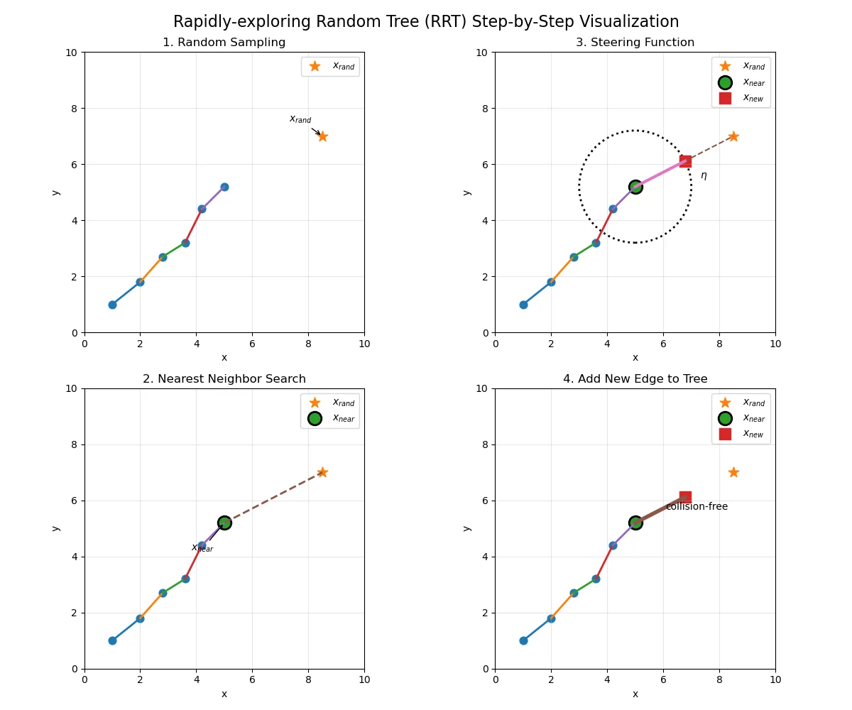
Figure 6: RRT Pseudocode Execution. A 4-panel step-by-step visualization of the RRT pseudocode in 2D. Panel 1: Show an existing tree and a newly sampled point x_rand. Panel 2: Highlight the Nearest Neighbor search, identifying x_near. Panel 3: Illustrate the Steering function generating x_new at a maximum distance $\eta$. Panel 4: Show the collision check confirming a free path and the new edge permanently added.

Figure 7: RRT Branching and Collision Checking. A similar visualization as Figure 6, highlighting branching and obstacle collision avoidance.
2.1.2 Characteristics and Voronoi Bias
The defining characteristic of the RRT algorithm is its space-filling exploration, which is governed by an inherent “Voronoi bias” [1]. Because the algorithm draws new states uniformly from the continuous space, the probability of selecting any specific vertex in the tree for expansion is strictly proportional to the continuous volume of its Voronoi region [1].
Vertices located on the frontier of the expanding tree naturally possess unbounded or significantly larger Voronoi cells compared to internal vertices, which are bounded tightly by their neighbors. Consequently, uniform global sampling naturally biases the tree to grow outward into unexplored regions of the configuration space, efficiently discovering paths without an explicit representation of obstacle boundaries [1].
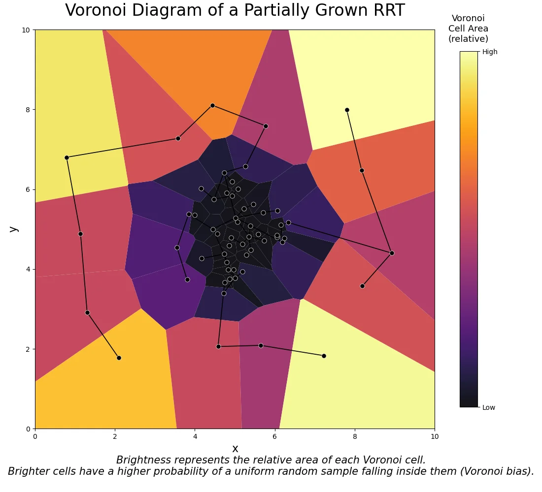
Figure 8: RRT Voronoi Bias. A Voronoi heatmap on a 2D space for a partially grown RRT tree. The cells of the Voronoi diagram corresponding to the tree’s vertices are colored using a brightness scale proportional to their area (e.g., larger frontier cells are intensely bright, while small internal cells are dark). The brightness represents the higher probability of a uniform sample falling into that cell, illustrating the Voronoi bias.
2.1.3 Complexity and Theoretical Guarantees
By avoiding explicit representation of the state space, the RRT algorithm drastically reduces the computational constraints associated with exact graph-search methods, particularly in higher dimensions.
-
Space Complexity: The space complexity of RRT is dictated by the graph size, requiring $O(n)$ memory where $n$ is the number of iterations (or samples). This linear relationship successfully bypasses the $O(k^d)$ exponential memory explosion typical of discrete grid searches in a $d$-dimensional space.
-
Time Complexity: The asymptotic time complexity of the algorithm is $O(n \log n + n \log^d m)$ [2], where $m$ is the number of obstacles in the environment. The $O(n \log n)$ term is derived from the nearest-neighbor search procedure. In fixed dimensions, finding the nearest neighbor takes $O(\log n)$ expected time using spatial data structures like K-D trees. While exact nearest-neighbor queries can degrade as dimensionality strictly increases, practical implementations utilize $\epsilon$-approximate nearest neighbor structures (such as balanced-box decomposition trees) to maintain sublinear $O(\log n + (1/\epsilon)^{d-1})$ query times in high-dimensional spaces [2]. The $O(\log^d m)$ term accounts for collision checking at each iteration.
The primary theoretical properties of the RRT algorithm are as follows:
-
Probabilistic Completeness (Theorem 16 [2]): RRT is mathematically proven to be probabilistically complete. For any robustly feasible path planning problem, as the number of vertices approaches infinity, the probability that the tree contains a valid path from the start to the goal region converges to one. The probability of failure decays to zero exponentially [2].
-
Non-Optimality (Theorem 33 [2]): While probabilistically complete, RRT lacks asymptotic optimality. The algorithm connects new samples strictly to their single nearest neighbor, which permanently locks in suboptimal local connections. Assuming the optimal path has a measure of zero, the probability that the cost of the path returned by RRT converges to the optimal cost $c^{*}$ is exactly zero. Therefore, standard RRT will almost surely converge to a suboptimal solution [2].
2.2 Achieving Optimality: Optimal RRT (RRT*)
2.2.1 Algorithm Overview and Pseudocode
The Optimal Rapidly-exploring Random Tree (RRT) algorithm [2] is an extension of the standard RRT designed to solve the optimal path planning problem. While it shares the incremental, single-query nature of RRT, it introduces two localized graph-modification operations to maintain a minimum-cost tree. The fundamental logic of RRT is defined by the following sequence of operations:
GENERATE_RRT*(x_init, K, Δt)
1   V ← {x_init}; E ← ∅;
2   for k = 1 to K do
3       x_rand ← RANDOM_STATE();
4       x_nearest ← NEAREST_NEIGHBOR((V, E), x_rand);
5       x_new ← STEER(x_nearest, x_rand, Δt);
6       if COLLISION_FREE(x_nearest, x_new) then
7           X_near ← NEAR((V, E), x_new, r(k));
8           V ← V ∪ {x_new};
9           x_min ← x_nearest; c_min ← Cost(x_nearest) + c(Line(x_nearest, x_new));
            // Connect along a minimum-cost path
10          foreach x_near ∈ X_near do
11              if COLLISION_FREE(x_near, x_new) ∧ Cost(x_near) + c(Line(x_near, x_new)) < c_min then
12                  x_min ← x_near;
13                  c_min ← Cost(x_near) + c(Line(x_near, x_new));
14          E ← E ∪ {(x_min, x_new)};
            // Rewire the tree
15          foreach x_near ∈ X_near do
16              if COLLISION_FREE(x_new, x_near) ∧ Cost(x_new) + c(Line(x_new, x_near)) < Cost(x_near) then
17                  x_parent ← Parent(x_near);
18                  E ← (E \ {(x_parent, x_near)}) ∪ {(x_new, x_near)};
19  Return G = (V, E);
The algorithm begins with the identical sampling (RANDOM_STATE), nearest-neighbor search (NEAREST_NEIGHBOR), and steering (STEER) procedures as the baseline RRT. However, once a valid $x_{new}$ is found, RRT* defines a localized neighborhood of existing vertices, $X_{near}$, within a specific radius $r(k)$ [2]. It then executes a two-step optimization. First, it evaluates all vertices in $X_{near}$ to identify the parent that provides the lowest total cost to reach $x_{new}$ from the root, connecting $x_{new}$ to that specific optimal parent instead of strictly defaulting to $x_{nearest}$. Second, it iterates through $X_{near}$ again to determine if routing any existing neighbor through the newly added $x_{new}$ yields a lower total cost than its current path. If a cheaper path is found, the existing edge is deleted and the neighbor is “rewired” to $x_{new}$ [2].
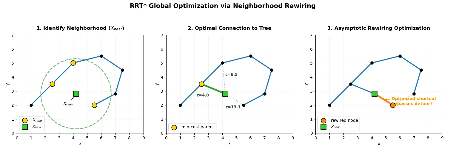
Figure 9: RRT* Rewiring Operations. Panel 1: Show a new node $x_{new}$ and a radius defining the set $X_{near}$. Panel 2: Highlight the “Connect along minimum-cost path” step, showing $x_{new}$ evaluating multiple neighbors to find the cheapest path back to the root. Panel 3: Illustrate the “Rewiring” step, showing an existing node disconnecting from its previous parent and re-attaching to $x_{new}$ to achieve a shorter path.
2.2.2 Characteristics: Random Geometric Graphs and Tree Morphology
The optimality of RRT* is derived from the theoretical properties of Random Geometric Graphs (RGGs) [2]. In RGGs, graph connectivity exhibits a phase transition dependent on the connection radius utilized [2]. Standard RRT fails to achieve optimality because it limits connections to a single nearest neighbor, permanently locking in suboptimal local connections. RRT* overcomes this by implicitly mimicking the connections of an RGG up to a specific radius.
A constant connection radius would result in an excessive number of connection attempts as the vertex density increases, destroying computational efficiency. To balance optimality with efficiency, RRT* employs a dynamically shrinking radius heuristic defined mathematically as [2]:
Block
where $n$ is the current number of vertices in the tree, $d$ is the dimensionality of the state space, and $\eta$ is the maximum steering step size. The constant $\gamma_{RRT*}$ is tuned based on the volume of the obstacle-free space, $\mu(X_{free})$, and the volume of a unit ball in $d$ dimensions, $\zeta_d$. This specific decay rate guarantees that the volume of the neighborhood evaluated shrinks proportionally to the increasing density of the tree [2]. Consequently, the average number of connections evaluated per iteration remains strictly proportional to $\log(n)$, maintaining the optimal connectivity properties of the graph without requiring an exhaustive $O(n)$ search at every step.
This rewiring mechanism fundamentally alters the macroscopic shape of the resulting tree. While standard RRT generates erratic, jagged branches due to its nearest-neighbor constraints, RRT* restructures itself into a shortest-path arborescence. In an obstacle-free space, this manifests as a distinct starburst pattern, with straight, optimal trajectories radiating directly outward from the root.
While the dynamic radius heuristic keeps local searches sublinear, the structural refinement of RRT* comes at a distinct computational cost. Standard RRT operates strictly as a rapid, greedy exploration tool; its single objective is to establish an initial feasible path, terminating the moment the goal region is pierced. Conversely, RRT* prioritizes asymptotic optimality, continuing to sample, evaluate near-neighbors, and rewrite existing edge topologies long after an initial solution is found. Because every iteration requires processing multiple candidate parents and executing cascade rewiring loops, RRT* exhibits significantly higher execution latency per sample than standard RRT. It trades immediate runtime execution speed for the guarantee that, given time, the discovered path will converge cleanly to the absolute theoretical minimum cost ($c^{*}$).
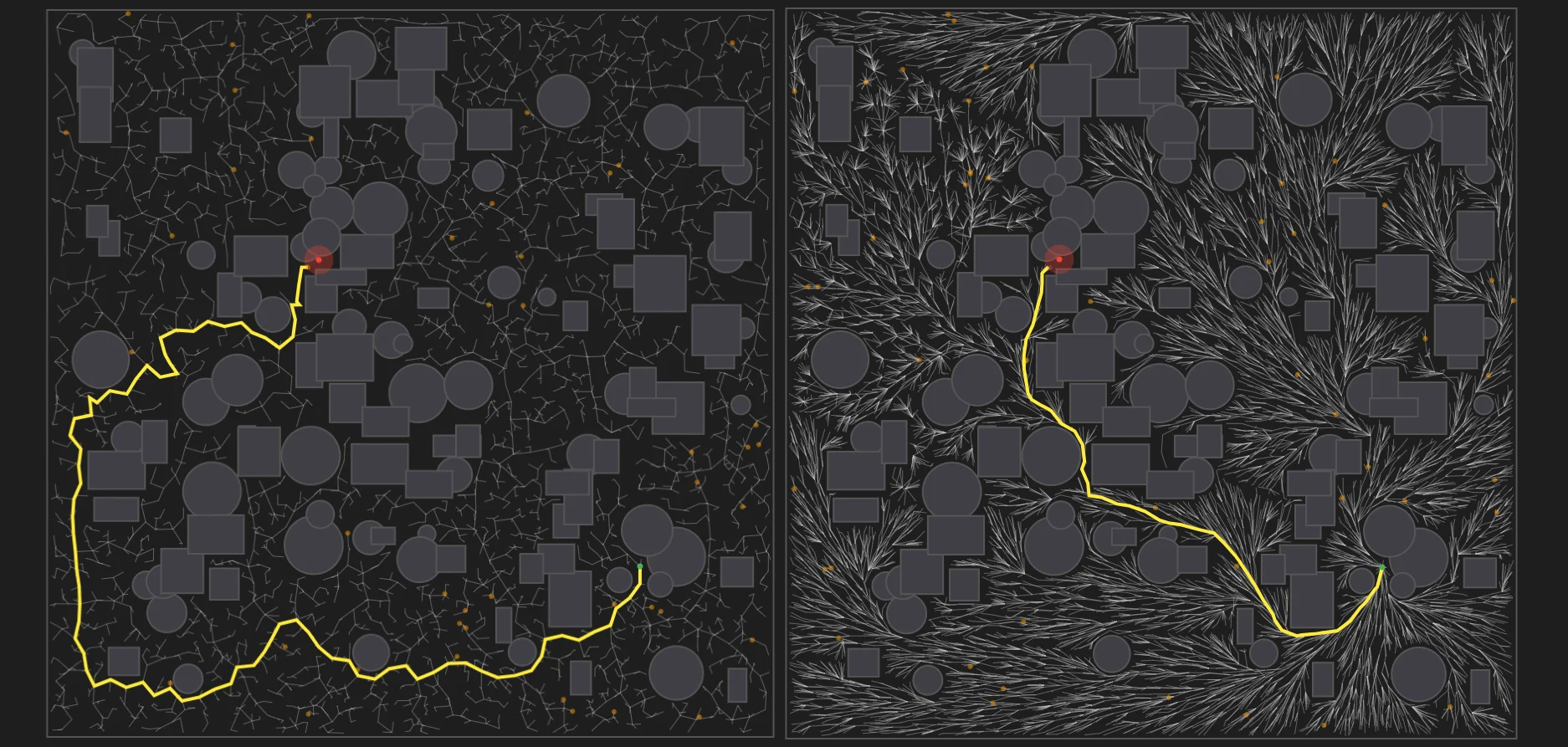
Figure 10: Tree Morphologies of RRT and RRT. The figure contrasts the jagged, suboptimal branches of a standard RRT, which prioritizes rapid feasibility, against the radial, straight-line arborescence of RRT after a large number of iterations (e.g., 10,000 samples) in a 2D obstacle-free environment, illustrating its continuous pursuit of asymptotic optimality at the expense of computational speed per iteration. Generated via RRT Playground [7].
2.2.3 Complexity and Theoretical Guarantees
By constraining the local neighborhood evaluations with the shrinking radius, RRT* maintains sub-quadratic computational complexity while drastically improving the theoretical guarantees over standard RRT.
-
Space Complexity: RRT* maintains a strict tree topology by replacing an existing edge for every rewiring operation. Because exactly one vertex and one final edge are added per iteration, the space complexity remains $O(n)$ [2].
-
Time Complexity: The asymptotic time complexity of RRT* is $O(n \log n)$ [2]. The
NEARprocedure can be executed in $O(\log n)$ expected time using appropriate spatial partitioning structures (such as balanced-box decomposition trees). Because the shrinking radius ensures the expected number of vertices returned byNEARis bounded by $O(\log n)$, the subsequent collision-checking and rewiring operations add only $O(\log n \log^d m)$ time per iteration, where $m$ is the number of obstacles. Therefore, the overall time complexity is preserved as asymptotically equivalent to the standard RRT [2].
The primary theoretical properties of the RRT* algorithm are established as follows:
-
Probabilistic Completeness (Theorem 23 [2]): Because RRT* shares the exact same vertex set as the standard RRT for identical random sequences, and ensures the graph remains a connected tree, it fundamentally inherits RRT’s probabilistic completeness. The probability that the RRT* tree contains a valid path to the goal converges to one as $n \to \infty$ [2].
-
Asymptotic Optimality (Theorem 38 [2]): RRT* mathematically guarantees almost-sure asymptotic optimality. Karaman and Frazzoli [2] rigorously prove that provided the constant $\gamma_{RRT^{*}}$ satisfies the bound $\gamma_{RRT^{*}} > (2(1+1/d))^{1/d}(\mu(X_{free})/\zeta_d)^{1/d}$, the cost of the best path returned by the algorithm converges almost surely to the absolute optimal cost $c^{*}$ as the number of samples approaches infinity. Furthermore, because the algorithm applies this localized rewiring globally across all uniform samples over time, RRT* does not merely optimize the path to a single goal region. Given infinite time, it theoretically constructs a complete shortest-path arborescence, formally discovering the absolute optimal path from the initial state $x_{start}$ to every other state within the reachable continuous space $X_{free}$.
2.3 Focusing the Search: Informed RRT*
2.3.1 Algorithm Overview and Pseudocode
While RRT* achieves asymptotic optimality, it does so by continuing to sample the entire global obstacle-free space even after an initial solution is found, effectively calculating the optimal path from the start state to every other state in the domain. Informed RRT* [3] addresses this inefficiency by introducing a heuristic-based focusing mechanism. Once an initial path is found, Informed RRT* restricts all subsequent sampling exclusively to the subset of states capable of improving the current solution [3].
For problems seeking to minimize path length in $\mathbb{R}^n$, the heuristic cost of a state $x$ is bounded by the Euclidean distance from the start to $x$, plus the distance from $x$ to the goal. The informed subset $X_{\hat{f}}$ is formally defined as a prolate hyperspheroid (a special hyperellipsoid) bounded by the cost of the best current solution, $c_{best}$ [3]:
Block
The algorithm operates identically to RRT*, with the exception of tracking $c_{best}$ and modifying the random state generation function:
INFORMED_RRT*(x_start, x_goal, K, Δt)
1   V ← {x_start}; E ← ∅; X_soln ← ∅;
2   c_best ← ∞
3   for k = 1 to K do
4       c_best ← min(Cost(x) for x in X_soln)
5       x_rand ← INFORMED_SAMPLE(x_start, x_goal, c_best)
6       x_nearest ← NEAREST_NEIGHBOR((V, E), x_rand)
7       x_new ← STEER(x_nearest, x_rand, Δt)
        // Standard RRT* collision checking and rewiring steps follow
8       if COLLISION_FREE(x_nearest, x_new) then
9           X_near ← NEAR((V, E), x_new, r(k))
10          V ← V ∪ {x_new}
            // Connect along minimum-cost path
11          // [Identical to RRT* Lines 9-14]
            // Rewire the tree
12          // [Identical to RRT* Lines 15-18]
13          if IN_GOAL_REGION(x_new) then
14              X_soln ← X_soln ∪ {x_new}
15  Return G = (V, E)
The INFORMED_SAMPLE procedure relies on a specific mathematical transformation to uniformly sample the heuristic subset rather than the entire global space:
INFORMED_SAMPLE(x_start, x_goal, c_best)
1   if c_best < ∞ then
2       c_min ←  || x_goal - x_start ||_2
3       x_centre ← (x_start + x_goal) / 2
4       C ← ROTATION_TO_WORLD_FRAME(x_start, x_goal)
5       L ← DIAG{c_best / 2, √(c_best^2 - c_min^2) / 2, ..., √(c_best^2 - c_min^2) / 2}
6       x_ball ← SAMPLE_UNIT_N_BALL()
7       x_rand ← (C * L * x_ball + x_centre) ∩ X_free
8   else
9       x_rand ← RANDOM_STATE_UNIFORM(X_free)
10  Return x_rand
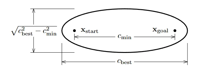
Figure 11: Heuristic Ellipsoidal Sampling. The heuristic sampling domain, , for a $\mathbb{R}^2$ problem seeking to minimize path length is an ellipse with the initial state, $x_{start}$, and the goal state, $x_{goal}$ as focal points. The shape of the ellipse depends on both the initial and goal states, the theoretical minimum cost between the two, $c_{min}$, and the cost of the best solution found to date, $c_{best}$. The eccentricity of the ellipse is given by $c_{min}/c_{best}$ [3].
2.3.2 Characteristics: Direct Ellipsoidal Sampling vs. Rejection Sampling
The primary challenge of focusing the search is efficiently generating samples within the $X_{\hat{f}}$ subset. A naive approach is rejection sampling, where points are drawn uniformly from a global bounding box and rejected if they fall outside the ellipse. However, the probability of improving a solution through rejection sampling decreases rapidly as state dimensionality $n$ increases or as the solution approaches the theoretical minimum $c_{min}$ [3]. If the bounding box is defined as a tight hyperrectangle around the prolate hyperspheroid, the probability of a uniform sample falling within the informed subset is $\zeta_n / 2^n$ (where $\zeta_n$ is the volume of a unit $n$-ball) [3]. In a 6-dimensional space, this yields a maximum success probability of merely 8% [3], rendering rejection sampling computationally prohibitive.
Informed RRT* bypasses this limitation via direct sampling. It first draws a sample uniformly from a unit $n$-ball, $x_{ball}$. The sample is scaled into the correct ellipsoidal proportions using the diagonal matrix $L$, which is derived from the Cholesky decomposition of the hyperellipsoid matrix [3]. The scaled point is then rotated to align with the transverse axis defined by $x_{start}$ and $x_{goal}$ using a rotation matrix $C \in SO(n)$ (solved as a Wahba problem) [3], and finally translated to the subset’s center $x_{centre}$. This direct transformation guarantees a uniform distribution strictly within the heuristic bounds, entirely bypassing the inefficiencies of high-dimensional rejection limits [3].
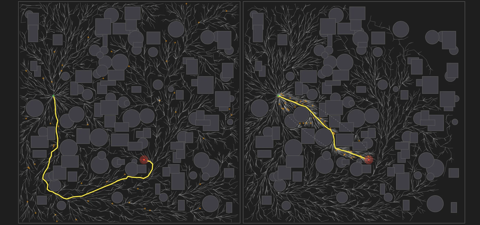
Figure 12: Tree Morphologies of RRT* vs. Informed RRT. Side-by-side comparison illustrating RRT continuing to sample globally after an initial solution is found, while Informed RRT* confines its dense branching strictly within the boundary of the bounding ellipse. Generated via RRT Playground [7].
2.3.3 Complexity and Theoretical Guarantees
Because Informed RRT* strictly inherits the core rewiring logic of RRT*, it maintains the same baseline asymptotic complexities, but with substantially reduced constant factors in practice.
-
Space Complexity: The space complexity remains bounded at $O(n)$. However, because fewer states are placed in regions that cannot improve the path, the tree maintains a more compact structure centered around the optimal path.
-
Time Complexity: The expected time complexity remains $O(n \log n)$ per iteration due to the spatial data structure queries required for the
NEARESTandNEARfunctions. The critical distinction is the shrinking radius calculation. In Informed RRT, the term $\mu(X_{free})$ used in the RRT radius calculation $\gamma_{RRT*} (\log(n)/n)^{1/d}$ is safely replaced by the measure of the informed subset, $\mu(X_{\hat{f}})$. As $c_{best}$ decreases, the volume of the search space shrinks [3], which systematically reduces the required connection radius and minimizes the number of collision-checking evaluations.
The theoretical properties of Informed RRT* mirror and extend upon RRT*:
-
Probabilistic Completeness and Asymptotic Optimality: Informed RRT* retains both the probabilistic completeness and almost-sure asymptotic optimality of RRT* because it preserves uniform sampling strictly within the subset containing all strictly better paths [3].
-
Theorem 1 (Obstacle-Free Linear Convergence) [3]: With the introduction of direct uniform sampling of the informed subset, the algorithm provides an explicit convergence rate. The expectation of the heuristic cost of a sample drawn from the hyperspheroid yields linear convergence. In the theoretical absence of obstacles, the cost of the best solution $c_{best}$ converges linearly to the theoretical minimum $c_{min}$ [3].
2.4 Unifying Discrete and Continuous Search: Batch Informed Trees (BIT*)
2.4.1 Algorithm Overview and Pseudocode
The algorithms discussed previously (RRT, RRT, and Informed RRT) process randomly generated states individually. Batch Informed Trees (BIT) [4] departs from this paradigm by unifying continuous sampling-based planning with exact discrete graph-search techniques, such as A and Lifelong Planning A* (LPA) [4]. BIT generates samples in batches and treats them as an implicit Random Geometric Graph (RGG). By searching this implicit RGG using heuristic estimates, BIT* evaluates states in a strictly ordered manner, bridging the gap between randomized space exploration and methodical dynamic programming.
The core logic of the BIT* algorithm relies on two queues: a vertex expansion queue ($Q_V$) and an edge evaluation queue ($Q_E$) [4]. The baseline procedure is defined by the following sequence of operations:
BIT*(x_start, x_goal)
1   V ← {x_start}; E ← ∅; X_samples ← {x_goal}
2   Q_E ← ∅; Q_V ← ∅; r ← ∞
3   repeat
4       if Q_E ≡ ∅ and Q_V ≡ ∅ then
5           PRUNE(g_T(x_goal))
6           X_samples ← X_samples ∪ SAMPLE(m, g_T(x_goal))
7           V_old ← V; Q_V ← V
8           r ← RADIUS( | V |  +  | X_samples | )
        // Expand vertices into the edge queue based on heuristic bounds
9       while BEST_QUEUE_VALUE(Q_V) ≤ BEST_QUEUE_VALUE(Q_E) do
10          EXPAND_VERTEX(BEST_IN_QUEUE(Q_V))
        // Process the best edge
11      (v_m, x_m) ← BEST_IN_QUEUE(Q_E)
12      Q_E ← Q_E \ {(v_m, x_m)}
        // Verify if the edge can improve the current best solution
13      if g_T(v_m) + c_hat(v_m, x_m) + h_hat(x_m) < g_T(x_goal) then
            // Check true collision status and exact edge cost
14          if g_T(v_m) + c(v_m, x_m) < g_T(x_m) then
15              if x_m ∈ V then
16                  E ← E \ {(v, x_m) ∈ E} // Rewire existing vertex
17              else
18                  X_samples ← X_samples \ {x_m}
19                  V ← V ∪ {x_m}; Q_V ← Q_V ∪ {x_m}
20              E ← E ∪ {(v_m, x_m)}
21              Q_E ← Q_E \ {(v, x_m) ∈ Q_E  |  g_T(v) + c_hat(v, x_m) ≥ g_T(x_m)}
22      else
23          Q_E ← ∅; Q_V ← ∅
24  until STOP
25  Return T = (V, E)
The algorithm begins a new batch by populating the free space with $m$ samples. Once an initial solution is found, the SAMPLE and PRUNE functions restrict all new samples and existing vertices strictly to the informed ellipsoidal subset, operating exactly as Informed RRT* [4]. The algorithm then updates the connection radius $r$ based on the new total sample count. Instead of connecting samples immediately, BIT* places existing tree vertices into $Q_V$. Vertices are expanded to populate $Q_E$ with potential edges. The edge in $Q_E$ with the lowest estimated total cost is extracted and evaluated. If the edge provides a shorter path to a target state, the exact cost is computed (including collision checking). If the edge remains valid and optimal, it is added to the tree, potentially rewiring existing connections. Once the queues are emptied, either because all useful edges have been evaluated or the remaining edges cannot improve the current solution, a new batch of $m$ samples is generated, and the process repeats.
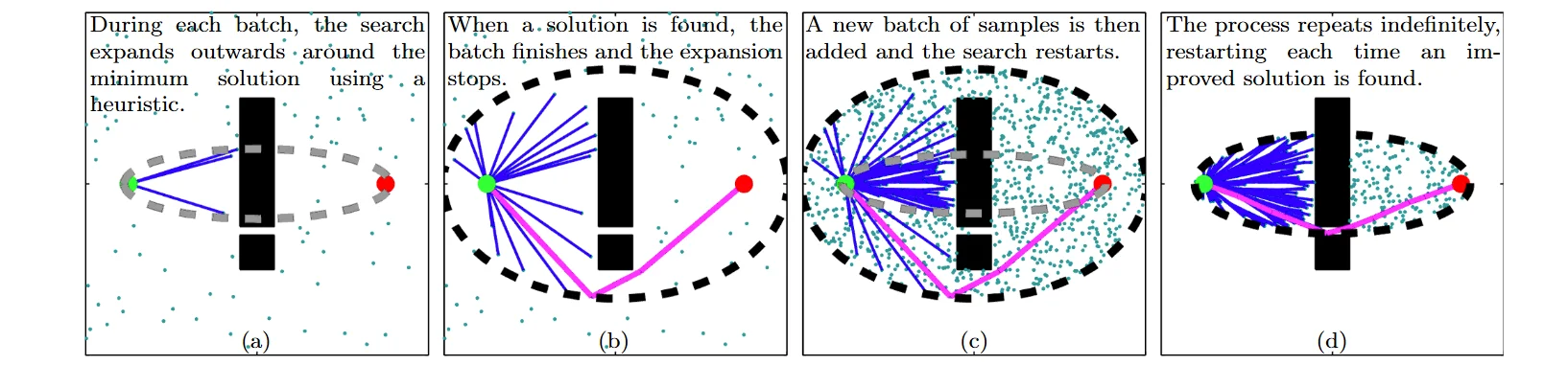
Figure 13: BIT* Informed Search Procedure. 4-panel illustration of the informed search procedure. Panel (a) shows the growing search of the first batch of samples. Panel (b) shows the first search ending when a solution is found. Panel (c) shows the search restarting on a denser graph after pruning and adding a second batch. Panel (d) shows the second search ending when an improved solution is found [4].
2.4.2 Characteristics: Implicit RGGs and Heuristic Ordering
The structural advancement of BIT* lies in its treatment of the planning domain as an implicit RGG [4]. In graph-based planning, building explicit connections between all sampled states is computationally prohibitive. By defining the edges implicitly via a distance boundary $r$, BIT* avoids computing or storing the full graph.
To navigate this implicit graph efficiently, BIT* introduces a heuristic ordering directly analogous to Lifelong Planning A* (LPA) [4]. BIT utilizes admissible heuristic functions to estimate the cost-to-come from the start state ($\hat{g}(x)$), the cost-to-go to the goal ($\hat{h}(x)$), and the cost of an individual edge ($\hat{c}(x,y)$). The edge queue $Q_E$ sorts potential connections based on their estimated total solution cost: $\hat{g}(v) + \hat{c}(v,x) + \hat{h}(x)$ [4].
This prioritization ensures that the algorithm delays the most computationally expensive operation in motion planning, evaluating the true edge cost $c(x,y)$, which requires continuous collision checking, until absolutely necessary. Edges are only checked for collisions if their heuristic cost suggests they are part of a path capable of improving the current best solution. Furthermore, by retaining samples across batches and processing them through incremental queues, BIT* systematically reuses previous collision-checking information [4].
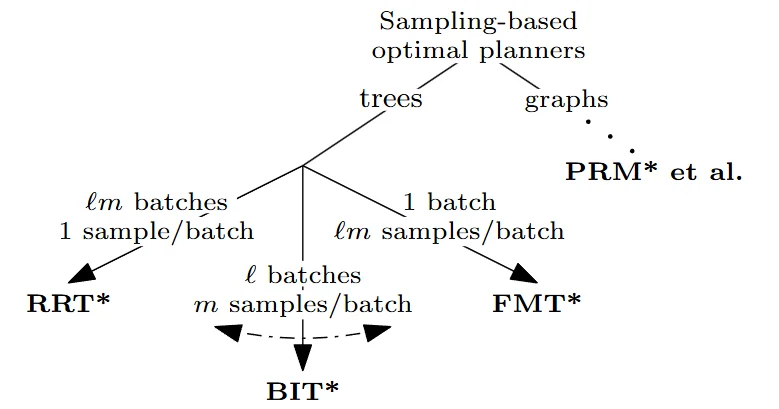
Figure 14: Taxonomy of Sampling-Based Optimal Planners. The visual illustrates the relationship between RRT* (1 sample per batch over infinite batches), FMT* ($m$ samples over 1 batch), and BIT* ($m$ samples per batch over infinite batches) [4].
2.4.3 Complexity and Theoretical Guarantees
BIT* combines the continuous scalability of sampling-based methods with the optimal search efficiency of discrete graph algorithms.
-
Space Complexity: By utilizing an implicit RGG representation, BIT* is not required to store the full operational graph in memory. For a total of $q$ samples generated across all batches, the space complexity is bounded strictly by $O(q)$ [4]. This linear memory footprint accounts for the explicitly verified tree vertices $ \mid V \mid $, the final tree edges $ \mid E \mid $, and the active unconnected samples tracked in $X_{samples}$. Pruning further restricts this space complexity in practice by systematically discarding samples and vertices that fall outside the heuristic bounds of the informed ellipsoidal subset.
-
Time Complexity: The execution time benefits substantially from the LPA* queue equivalence and the avoidance of exhaustive global searches [4]. Extracting the required geometric proximity constraints is managed by spatial data structures (such as k-d trees), which execute nearest-neighbor queries in $O(\log q)$ expected time. The worst-case time complexity to compute the optimal paths over the continuously expanding explicit graph is bounded by $O( \mid V \mid \log \mid V \mid + \mid E \mid )$. Furthermore, by sorting the processing queues using the admissible heuristic estimate $\hat{c}(x,y)$ instead of the true edge cost $c(x,y)$, BIT* delays and minimizes $O(\log^d m)$ collision-checking queries, ensuring sub-quadratic computational scaling as batch iterations accumulate [4].
The theoretical guarantees of BIT* map directly to the foundational proofs of RRT*:
- Probabilistic Completeness and Asymptotic Optimality (Theorem 1 [4]): BIT* is mathematically proven to be almost-surely asymptotically optimal, converging to the optimal solution $s^{*}$ with probability one as the number of samples approaches infinity [4]. The proof relies on a direct reduction to RRT. For any given sequence of $q$ uniformly distributed random samples, RRT considers all edges involving earlier samples up to a specific connection radius $r_q$. BIT* processes that exact same sequence of samples in batches. For any sample within a batch, BIT* considers all edges involving samples from the same or earlier batches up to the identical radius $r_q$ [4]. Because BIT* maintains uniform sample density in the subproblem and evaluates a superset of the edge connections defined by RRT* for a given sequence, BIT* inherently satisfies the required conditions for almost-sure asymptotic optimality [4].
3. Experiments
To empirically validate the theoretical advancements discussed in this report, an experimental suite was conducted utilizing the RRT Playground simulation environment. The experiments were designed to isolate and evaluate the algorithms across three continuous motion planning scenarios: an unobstructed baseline, a clustered obstacle field, and a constrained maze geometry.
The primary metrics evaluated across all algorithms (RRT, RRT, Informed RRT, and BIT*) are the execution time and iterations required to discover an initial feasible path, the final optimal path cost ($c_{best}$) achieved within the allocated processing limit, and the memory footprint denoted by the explicit vertex ($ \mid V \mid $) and edge ($ \mid E \mid $) counts.
3.1 Experiment 1: Morphology & Baseline Test (Empty Environment)
Objective: To establish the baseline convergence rate without obstacle interference and visually validate the theoretical search morphologies (Voronoi arborescence, ellipsoidal bounding, and implicit graph sparsity) discussed in Section 2.
![]()
Figure 15: Algorithm Morphologies in an Empty Environment. Top-Left: RRT (Baseline tree). Top-Right: RRT* (Global arborescence). Bottom-Left: Informed RRT* (Ellipsoidal bounding). Bottom-Right: BIT* (Implicit sparse graph).
Table 1: Empty Environment Results
| Algorithm | Init Time (s) | Init Iters | Init Cost | Final Time (s) | Final Iters | Final Cost | Final Vertices | Final Edges |
|---|---|---|---|---|---|---|---|---|
| RRT | 0.122 | 289 | 768.00 | 0.122 | 289 | 768.00 | 290 | 289 |
| RRT* | 0.123 | 289 | 736.70 | 4.855 | 5289 | 687.97 | 5290 | 5289 |
| IRRT* | 0.123 | 289 | 736.70 | 4.887 | 5289 | 619.47 | 5290 | 5289 |
| BIT* | 0.695 | 1439 | 744.78 | 5.443 | 6439 | 624.33 | 12 | 11 |
Analysis: In an unobstructed continuous space, the Euclidean heuristic aligns with the true path cost. Because standard RRT, RRT, and Informed RRT (IRRT*) utilize identical initial uniform sampling, they reached the goal region at 289 iterations (0.12 seconds).
The post-discovery optimization phase illustrates the structural differences among the algorithms. Given 4.8 seconds of optimization, IRRT* achieved the lowest cost (619.47) by directly sampling within its bounding ellipsoid. Visually, RRT* constructed a dense global arborescence covering the coordinate space, while IRRT* restricted its 5,290 vertices strictly to the defined heuristic bounds.
BIT* demonstrated lower memory usage. Relying on an implicit Random Geometric Graph and an ordered evaluation queue, it achieved convergence (624.33) while storing an explicit tree of 12 vertices, producing a direct sequence of edges without evaluating unconnected regions of the state space.
3.2 Experiment 2: The Clutter Benchmark (Random Forest)
Objective: To evaluate the algorithms’ computational efficiency under collision-checking loads. Complex obstacle arrangements introduce local minima, testing heuristic convergence rates.
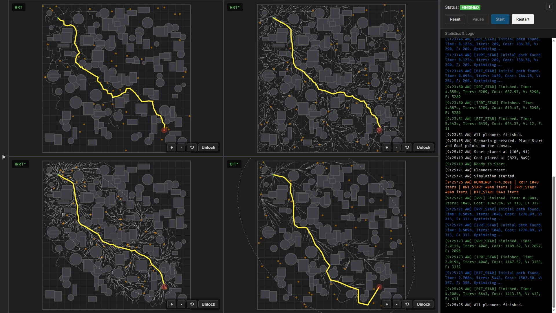
Figure 16: Algorithm Performance in a Random Forest Environment, demonstrating path optimization and state-space pruning under collision-checking conditions.
Table 2: Random Forest Environment Results
| Algorithm | Init Time (s) | Init Iters | Init Cost | Final Time (s) | Final Iters | Final Cost | Final Vertices | Final Edges |
|---|---|---|---|---|---|---|---|---|
| RRT | 0.508 | 1048 | 1342.64 | 0.508 | 1048 | 1342.64 | 313 | 312 |
| RRT* | 0.509 | 1048 | 1276.09 | 2.011 | 4048 | 1189.62 | 2897 | 2896 |
| IRRT* | 0.509 | 1048 | 1276.09 | 2.019 | 4048 | 1147.52 | 3153 | 3152 |
| BIT* | 2.708 | 5443 | 1502.50 | 4.208 | 8443 | 1413.78 | 412 | 411 |
Analysis: The introduction of scattered, overlapping obstacles increases the computational requirements of the nearest-neighbor and steering functions. Standard RRT discovered a sub-optimal path (cost: 1342.64) and terminated. IRRT* reduced the path cost to 1147.52 by concentrating its sampling within the free space situated between the start and goal states.
BIT* required more iterations (5443) and time (2.708s) to discover an initial path. This is attributed to the computational overhead of its batching phase and its reliance on a heuristic queue, which can temporarily prioritize obstructed direct paths over necessary deviations. However, it maintained lower memory allocation, holding 412 explicit vertices compared to IRRT*’s 3,153.
3.3 Experiment 3: The Narrow Passage & Heuristic Trap (Maze)
Objective: To evaluate the algorithms’ capacity for long-horizon planning in constrained spaces where the Euclidean heuristic contradicts the spatial geometry, necessitating back-tracking.
Note: The global iteration limit was increased to 25,000 for this benchmark.
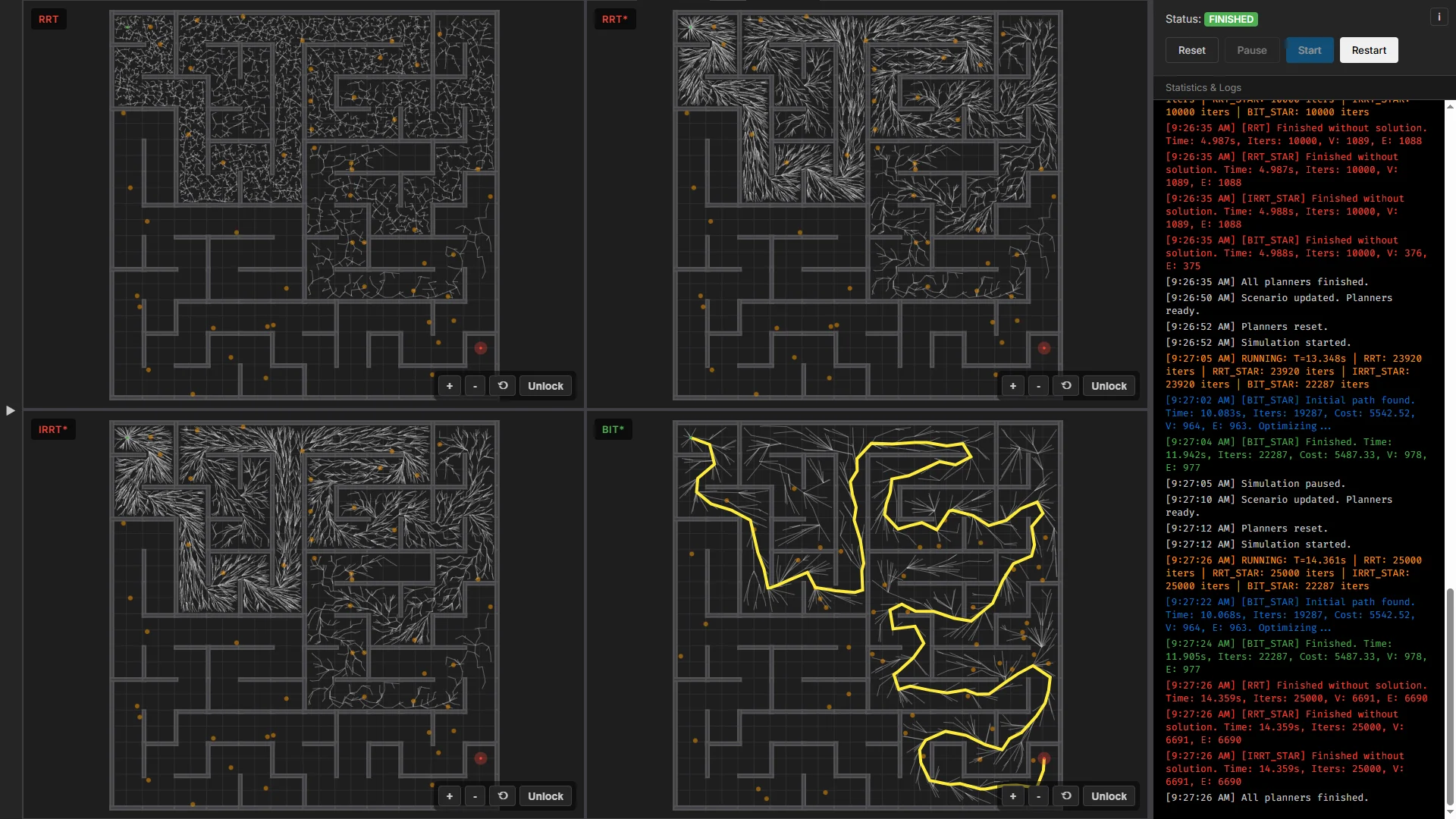
Figure 17: Algorithm Performance in a Maze Environment. RRT, RRT, and Informed RRT fail to traverse the narrow corridors within the iteration limit, while BIT* successfully calculates a feasible path.
Table 3: Maze Environment Results
| Algorithm | Init Time (s) | Init Iters | Init Cost | Final Time (s) | Final Iters | Final Cost | Final Vertices | Final Edges |
|---|---|---|---|---|---|---|---|---|
| RRT | N/A | N/A | N/A | 14.359 | 25000 | Failed | 6691 | 6690 |
| RRT* | N/A | N/A | N/A | 14.359 | 25000 | Failed | 6691 | 6690 |
| IRRT* | N/A | N/A | N/A | 14.359 | 25000 | Failed | 6691 | 6690 |
| BIT* | 10.068 | 19287 | 5542.52 | 11.905 | 22287 | 5487.33 | 978 | 977 |
Analysis: The maze environment highlights the limitations of uniform global sampling for long-horizon planning. Standard RRT, RRT, and IRRT did not find an initial solution within the 25,000 iteration limit. The probability of uniform samples aligning sequentially through the narrow corridors is low, causing the baseline trees to densely populate local regions without progressing toward the goal. Because IRRT* never discovered an initial path, it did not construct a bounding ellipse, operating identically to standard RRT*.
Conversely, BIT* successfully navigated the maze. It discovered an initial path at 10.068s (19,287 iterations) and optimized it to a final cost of 5487.33. By processing samples in batches and treating them as an implicit graph, BIT* utilized its ordered search queue to systematically evaluate edges. This approach enabled the algorithm to sustain the long-horizon planning required to traverse the narrow passages rather than relying purely on the probability of sequential state expansion.
4. Conclusion
This report has detailed the theoretical and algorithmic progression of sampling-based motion planning methods, tracking the evolution from rapid feasible search to highly efficient optimal search. Traditional discrete graph-search methods fail in high-dimensional continuous spaces due to the curse of dimensionality. The baseline randomized approach, RRT, successfully circumvents this by utilizing uniform random sampling to rapidly explore the space, providing probabilistic completeness but yielding inherently suboptimal paths.
To bridge the gap to true optimal planning, RRT* introduces a local rewiring mechanism built on Random Geometric Graph theory. By defining a dynamically shrinking connection radius that evaluates nearby candidates without violating computational constraints, RRT* achieves almost-sure asymptotic optimality. To refine this approach, Informed RRT* leverages direct sampling of a heuristically defined prolate hyperspheroid, confining the algorithm’s global exploration strictly to the subset of states that can improve the current path, drastically accelerating convergence.
Finally, BIT* represents a paradigm shift by treating batches of samples as an implicit RGG and applying a heuristically ordered search analogous to LPA*. This ordered exploration avoids the exhaustive collision checking of unpromising edges, unifying the continuous scalability of randomized sampling with the meticulous efficiency of discrete dynamic programming. Planned experiments using 2D Maze and Random Forest environments will empirically validate how these theoretical advancements combine to resolve complex continuous motion planning queries efficiently and optimally.
References
- [1] LaValle, S. M. (1998). Rapidly-Exploring Random Trees: A New Tool for Path Planning.
- [2] Karaman, S., & Frazzoli, E. (2011). Sampling-based Algorithms for Optimal Motion Planning.
- [3] Gammell, J. D., Srinivasa, S. S., & Barfoot, T. D. (2014). Informed RRT*: Optimal Sampling-based Path Planning Focused via Direct Sampling of an Admissible Ellipsoidal Heuristic.
- [4] Gammell, J. D., Srinivasa, S. S., & Barfoot, T. D. (2015). Batch Informed Trees (BIT*): Sampling-based Optimal Planning via the Heuristically Guided Search of Implicit Random Geometric Graphs.
- [5] Koberstein, A., & Schocke, K. O. (2017). Multi-Agent Route Planning in Grid-Based Storage Systems.
- [6] Borington. (n.d.). A* (A star) vs Dijkstra’s algorithm pathfinding grid visualization - JavaScript. YouTube.
- [7] Pham-Duc, Duy (n.d.). RRT Playground. GitHub Pages.