Planar Four Wheel Model with Wheel Dynamics and Weight Transfer
Table of Content
Block
Prologue
Alright so I’m gonna be honest here, even though I’ve found these wonderful references that helped me immensely, I’m still not confident enough to code up another simulator after duy-phamduc68/Planar-Dynamic-Car-Model, which if you need more context, I recommend you checking out this post: Conclusion of the Macro Monster Car Physics Journey.
Nevertheless I still do want to get a feel for it, and I do have a differential equations course that require 2 project assignments so might as well. (plus, I just got Assetto Corsa on sale, wanted to flex it here, probably gonna make a dedicated post for it, mostly to take pictures, best $3 ever though).
So, what I’m gonna do from this post, is deriving the Planar Four Wheel Model with Wheel Dynamics and Weight Transfer from a UC Berkeley PhD thesis of Jon Matthew Gonzales, 2018. Specifically Section 2. of the thesis, and then run some qualitative experiments through code, then try my best to replicate the experiments in Assetto Corsa.
A. Vehicle Model Derivation
Direct citations:
- Section 2.1: Introduction (Pages 6-7): This defines the global, vehicle-fixed ($e^v$), and tire-fixed ($e^t$) coordinate systems. Understanding these frames is essential before looking at the coordinate transformation equations.
- Section 2.4: Slip angle and slip ratio (Pages 10-14): This section derives the kinematics. It shows exactly how to calculate the longitudinal ($v_x$) and lateral ($v_y$) velocities for each individual tire based on the vehicle’s center of mass and yaw rate. It also provides the formulas for the tire slip angles ($\alpha$) and slip ratios ($\sigma, \kappa$).
- Section 2.4: Combined Slip Models (Page 18): This is where the kinematic slip velocities are converted into actual tire forces. It outlines the math for the normalized combined slip ($s$) and shows how it plugs into the Pacejka Magic Formula to get $F_{x’}$ and $F_{y’}$ in the tire frame.
- Section 2.4: Planar Four-Wheel Model with Wheel Dynamics (Pages 21-22): This core section provides the primary differential equations for the chassis velocities ($\dot{v}_x, \dot{v}_y, \dot{r}$) and the wheel rotational dynamics ($\dot{\omega}$). It also contains the specific coordinate transformations needed to project the front tire forces back into the vehicle frame.
- Section 2.4: Four-Wheel Model Load Transfer (Pages 22-25): This section gives us what we need to solve the tire force equations, the dynamic normal force ($F_z$) acting on each wheel. This section uses the balance of linear and angular momentum, plus a vertical deformation constraint, to derive the $F_z$ formulas for all four wheels.
1. System States and Inputs
The model considers the chassis velocities, yaw rate, and the independent rotational speeds of all four wheels.
- State Vector: $z = [\begin{matrix}v_x & v_y & r & \omega^{fl} & \omega^{fr} & \omega^{rl} & \omega^{rr}\end{matrix}]^\top$
- Input Vector: $u = [\begin{matrix}\delta & T^{rr} & T^{rl}\end{matrix}]^\top$
2. Core Differential Equations (Equations of Motion)
These equations define how the vehicle state evolves over time. They account for the mass $m$, yaw moment of inertia $I_z$, wheel moment of inertia $I_w$, and wheel radius $R$.
Chassis Dynamics:
Block
Wheel Rotational Dynamics:
Block
3. Coordinate Transformations (Force)
Because the front wheels are steered by angle $\delta$, the forces generated in the local tire frame (denoted by a tick, like $x’$ or $y’$) must be projected back into the vehicle’s reference frame. The rear wheels are unsteered, so their frames align with the vehicle frame.
Front Wheels ($* \in {r, l}$):
Block
Rear Wheels:
Block
4. Wheel Kinematics (Velocities)
To determine slip, the system must calculate the longitudinal and lateral velocity at the center of each wheel patch in the vehicle frame, using yaw rate $r$ (noted as $\omega_z$ in the text) and distances $c$, $L_f$, and $L_r$.
Longitudinal Components:
Block
Lateral Components:
Block
Projection into the Tire Frame:
Just like forces, these velocities must be rotated into the local tire frame for the front wheels:
Block
5. Combined Slip Formulations
Using the velocities in the tire frame, the model computes the normalized longitudinal slip ($s_{x’}$), lateral slip ($s_{y’}$), and the combined slip magnitude ($s$).
Block
Block
6. Combined Slip Tire Model (Pacejka Magic Formula)
The tire forces in the local frame are calculated using the slip definitions and Pacejka curve parameters ($B, C, D$), constrained by the friction coefficient $\mu$ and the dynamic normal force $F_z$.
Block
7. Normal Forces (Dynamic Load Transfer)
Finally, to provide $F_z$ for the tire model above, the vehicle model calculates weight transfer based on the total planar forces ($F_X$ and $F_Y$) and the center of gravity height $h$.
Total Planar Forces:
Block
Normal Force per Wheel:
Block
B. Qualitative Experiments
Because we don’t really have access to academic / industry standard validation tools such as CarSim (proprietary, used in the UC Berkeley thesis), I’ve decided to run simple scenario experiments using known parameters and configuration from the main reference and some other sources for the vehicle parameters.
More specifically, in the UC Berkeley thesis, they employ discretization by Euler’s method at $dt = 0.01s$ (10ms), but the parameters of the vehicle is not consistent nor enough to be able to reproduce their results, thus, I came to a different reference, a Master’s thesis from Chalmers University of Technology:
- A Methodology for Identification of Magic Formula Tire Model Parameters from In-Vehicle Measurements
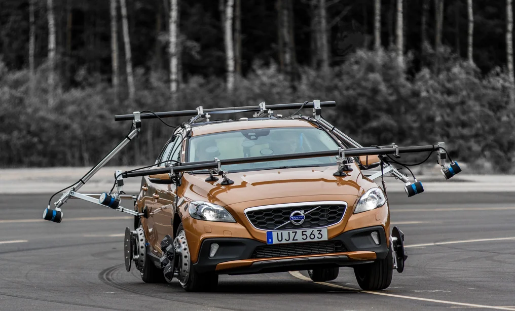
They performed their research on a Volvo V40. Their work use the VI-CarRealTime Simulator which is also a proprietary software.
1. Parameters Validation
In the above source, we actually don’t have exact parameters for the vehicle model, but we was able to confirm certain components of the Volvo V40. This allowed me to combine the exact data extracted from the document with the real-world OEM (Original Equipment Manufacturer) specifications for the 2013 Volvo V40 Cross Country in their experiment to derive a reasonable parameters set. More specifically:
1.1. Parameters Validated from the Master’s Thesis Document
- Vehicle Model (2013 Volvo V40 CC): The vehicle that was chosen for physical testing was a 2013 Volvo V40 CC.
- Tire Specification (Michelin Primacy HP 225/50R17): The tire that was chosen for testing was the Michelin Primacy HP 225/50R17.
- Wheel Radius ($R = 0.327$ m): The parameter fitting tool’s interface defines the unloaded radius ($R_0$) as 0.327 meters.
- Friction Coefficient ($\mu = 1.1$): The peak friction coefficient ($\mu_y$) is shown peaking between 1.1 and 1.2 for standard normal loads.
1.2. Parameters Validated from External Automotive Databases
Since the thesis omitted raw chassis dimensions, these were validated using real-world OEM specifications for the 2013 Volvo V40 Cross Country:
-
Wheelbase ($L_f$ and $L_r$): The official wheelbase for the 2013 V40 CC is 2.647 meters (2647 mm). Using a standard 56/44 transverse-engine weight distribution, this splits into $L_f = 1.15$ m and $L_r = 1.497$ m.
- Validation reference: AutoEvolution: Volvo V40 Cross Country 2012 Specs
-
Track Width ($c = 0.776$ m): The official front track width is 1.552 meters (1552 mm). The parameter $c$ in the vehicle model requires the half-track width, which perfectly halves to 0.776 meters.
- Validation reference: Automoli Technical Data: V40 CC Dimensions
-
Mass ($m = 1600$ kg): The unladen (curb) weight of the V40 CC ranges from 1359 kg to 1536 kg depending on the exact engine block (e.g., T4 vs D3/D4). Adding approximately 100-150 kg accounts for the driver and the massive exterior camera booms, wheel force transducers, and interior IMU boxes used in the experiment.
- Validation reference: UltimateSpecs: V40 CC Weights and Dimensions
1.3. Parameters Based on Standard Vehicle Dynamics Estimations
Because manufacturers rarely publish proprietary suspension geometries or dynamic inertias, these parameters use standard, mathematically accepted approximations for a 1600 kg compact hatchback:
- Center of Gravity Height ($h = 0.55$ m): A CG height of 500mm to 550mm is the universally accepted standard estimate for modern hatchbacks and crossovers in Pacejka tire modeling.
- Yaw Moment of Inertia ($I_z = 2700$ kg·m²): Often calculated using the standard approximation formula $I_z \approx m \times L_f \times L_r$. ($1600 \times 1.15 \times 1.497 \approx 2754$).
- Wheel Inertia ($I_w = 1.5$ kg·m²): A standard rotating inertia estimate for a 17-inch alloy wheel paired with a 225/50R17 tire and brake rotor assembly.
2. Code Implementation
We implement the vehicle model in Python code and plug in the parameters (the experiments were ran on a Colab notebook).
2.1. Standalone Vehicle Model
from __future__ import annotations

from dataclasses import dataclass
from typing import Iterable, Tuple, Union, Dict, Any

import numpy as np


ArrayLike = Union[float, Iterable[float], np.ndarray]
WHEEL_ORDER = ("fl", "fr", "rl", "rr")
EPS = 1e-9


def _as_4(x: ArrayLike, name: str) -> np.ndarray:
    arr = np.asarray(x, dtype=float)
    if arr.ndim == 0:
        return np.full(4, float(arr), dtype=float)
    arr = arr.reshape(-1)
    if arr.size != 4:
        raise ValueError(f"{name} must be a scalar or length-4 iterable.")
    return arr.astype(float, copy=False)


def _safe_denominator(x: float, eps: float = EPS) -> float:
    if abs(x) >= eps:
        return x
    return eps if x >= 0.0 else -eps


@dataclass
class VehicleParams:
    """
    Parameters for the 7-state combined-slip vehicle model.

    State vector:
        [vx, vy, r, omega_fl, omega_fr, omega_rl, omega_rr]

    Input vector:
        [delta, T_rr, T_rl]

    Notes:
        - B, C, D, mu may be scalar or length-4, ordered as:
          [fl, fr, rl, rr]
        - dt is fixed Euler step size in seconds.
        - The load-transfer equations are algebraically coupled to the tire
          forces; this implementation resolves them with fixed-point iteration.
    """

    m: float
    Iz: float
    Iw: float
    R: float
    Lf: float
    Lr: float
    c: float
    h: float
    B: ArrayLike
    C: ArrayLike
    D: ArrayLike
    mu: ArrayLike
    g: float = 9.81
    dt: float = 0.01
    load_transfer_iterations: int = 8
    load_transfer_tol: float = 1e-10

    def __post_init__(self) -> None:
        if self.m <= 0 or self.Iz <= 0 or self.Iw <= 0 or self.R <= 0:
            raise ValueError("m, Iz, Iw, and R must be positive.")
        if self.Lf < 0 or self.Lr < 0 or self.c <= 0 or self.h < 0:
            raise ValueError("Lf, Lr, c, h must be nonnegative, with c > 0.")
        if self.dt <= 0:
            raise ValueError("dt must be positive.")
        if self.load_transfer_iterations < 0:
            raise ValueError("load_transfer_iterations must be nonnegative.")

        self.B = _as_4(self.B, "B")
        self.C = _as_4(self.C, "C")
        self.D = _as_4(self.D, "D")
        self.mu = _as_4(self.mu, "mu")


@dataclass
class VehicleState:
    vx: float
    vy: float
    r: float
    omega_fl: float
    omega_fr: float
    omega_rl: float
    omega_rr: float

    def as_array(self) -> np.ndarray:
        return np.array(
            [
                self.vx,
                self.vy,
                self.r,
                self.omega_fl,
                self.omega_fr,
                self.omega_rl,
                self.omega_rr,
            ],
            dtype=float,
        )

    @classmethod
    def from_array(cls, x: ArrayLike) -> "VehicleState":
        arr = np.asarray(x, dtype=float).reshape(-1)
        if arr.size != 7:
            raise ValueError("State must have length 7.")
        return cls(*map(float, arr.tolist()))


@dataclass
class ControlInput:
    delta: float
    T_rr: float
    T_rl: float

    def as_array(self) -> np.ndarray:
        return np.array([self.delta, self.T_rr, self.T_rl], dtype=float)

    @classmethod
    def from_array(cls, u: ArrayLike) -> "ControlInput":
        arr = np.asarray(u, dtype=float).reshape(-1)
        if arr.size != 3:
            raise ValueError("Control input must have length 3.")
        return cls(*map(float, arr.tolist()))


class CombinedSlipVehicleModel:
    """
    Exact numerical translation of the provided 7-state model.

    Public API:
        - derivatives(state, control) -> np.ndarray shape (7,)
        - step(state, control) -> VehicleState
        - step_array(x, u) -> np.ndarray shape (7,)
        - eval_forces(state, control) -> dict of intermediate values
    """

    def __init__(self, params: VehicleParams):
        self.p = params

    def _wheel_center_velocities(self, state: np.ndarray) -> Dict[str, Tuple[float, float]]:
        vx, vy, r = float(state[0]), float(state[1]), float(state[2])

        # Vehicle-frame wheel center velocities
        vx_fr = vx + r * self.p.c
        vx_fl = vx - r * self.p.c
        vx_rr = vx + r * self.p.c
        vx_rl = vx - r * self.p.c

        vy_fr = vy + r * self.p.Lf
        vy_fl = vy + r * self.p.Lf
        vy_rr = vy - r * self.p.Lr
        vy_rl = vy - r * self.p.Lr

        return {
            "fr": (vx_fr, vy_fr),
            "fl": (vx_fl, vy_fl),
            "rr": (vx_rr, vy_rr),
            "rl": (vx_rl, vy_rl),
        }

    def _tire_frame_velocities(
        self, wheel_vel_vehicle: Dict[str, Tuple[float, float]], delta: float
    ) -> Dict[str, Tuple[float, float]]:
        c = float(np.cos(delta))
        s = float(np.sin(delta))

        out: Dict[str, Tuple[float, float]] = {}

        # Front wheels: rotate into tire frame.
        for w in ("fl", "fr"):
            vx_v, vy_v = wheel_vel_vehicle[w]
            vx_t = vx_v * c + vy_v * s
            vy_t = -vx_v * s + vy_v * c
            out[w] = (float(vx_t), float(vy_t))

        # Rear wheels: tire frame aligned with vehicle frame.
        out["rl"] = wheel_vel_vehicle["rl"]
        out["rr"] = wheel_vel_vehicle["rr"]
        return out

    def _slip_components(
        self, vx_t: float, vy_t: float, omega: float
    ) -> Tuple[float, float, float]:
        omega_r = omega * self.p.R
        if vx_t >= omega_r:
            sx = (omega_r - vx_t) / _safe_denominator(vx_t)
        else:
            sx = (omega_r - vx_t) / _safe_denominator(omega_r)
        sy = vy_t / _safe_denominator(omega_r)
        s = float(np.sqrt(sx * sx + sy * sy))
        return float(sx), float(sy), s

    def _combined_slip_force(
            self, wheel_index: int, Fz: float, sx: float, sy: float
        ) -> Tuple[float, float]:
            mu = float(self.p.mu[wheel_index])
            B = float(self.p.B[wheel_index])
            C = float(self.p.C[wheel_index])
            D = float(self.p.D[wheel_index])

            s = float(np.sqrt(sx * sx + sy * sy))
            if s <= EPS or Fz <= 0.0:
                return 0.0, 0.0

            # Removed the negative sign! This represents the magnitude of the grip.
            common = mu * Fz * D * float(np.sin(C * np.arctan(B * s)))

            # Longitudinal force aligns with longitudinal slip (positive slip = forward force)
            Fx_t = common * (sx / s)

            # Lateral force OPPOSES lateral slip (resists sliding)
            Fy_t = -common * (sy / s)

            return float(Fx_t), float(Fy_t)

    def _rotate_tire_forces_to_vehicle(
        self, wheel: str, Fx_t: float, Fy_t: float, delta: float
    ) -> Tuple[float, float]:
        if wheel in ("fl", "fr"):
            c = float(np.cos(delta))
            s = float(np.sin(delta))
            Fx = Fx_t * c - Fy_t * s
            Fy = Fx_t * s + Fy_t * c
            return float(Fx), float(Fy)
        return float(Fx_t), float(Fy_t)

    def _normal_forces(self, FX: float, FY: float) -> np.ndarray:
        p = self.p
        denom = 4.0 * p.c * (p.Lf + p.Lr)
        if abs(denom) < EPS:
            raise ZeroDivisionError("Invalid geometry: 4*c*(Lf+Lr) is too small.")

        Fz_fl = (
            2.0 * p.Lr * p.c * p.g * p.m
            - 2.0 * p.c * p.h * FX
            - p.h * (p.Lf + p.Lr) * FY
        ) / denom
        Fz_fr = (
            2.0 * p.Lr * p.c * p.g * p.m
            - 2.0 * p.c * p.h * FX
            + p.h * (p.Lf + p.Lr) * FY
        ) / denom
        Fz_rl = (
            2.0 * p.Lf * p.c * p.g * p.m
            + 2.0 * p.c * p.h * FX
            - p.h * (p.Lf + p.Lr) * FY
        ) / denom
        Fz_rr = (
            2.0 * p.Lf * p.c * p.g * p.m
            + 2.0 * p.c * p.h * FX
            + p.h * (p.Lf + p.Lr) * FY
        ) / denom

        return np.array([Fz_fl, Fz_fr, Fz_rl, Fz_rr], dtype=float)

    def eval_forces(self, state: ArrayLike, control: ArrayLike) -> Dict[str, Any]:
        x = np.asarray(state, dtype=float).reshape(-1)
        u = np.asarray(control, dtype=float).reshape(-1)
        if x.size != 7:
            raise ValueError("State must have length 7.")
        if u.size != 3:
            raise ValueError("Control input must have length 3.")

        delta = float(u[0])
        T_rr = float(u[1])
        T_rl = float(u[2])

        wheel_vel_vehicle = self._wheel_center_velocities(x)
        wheel_vel_tire = self._tire_frame_velocities(wheel_vel_vehicle, delta)

        p = self.p
        if abs(p.Lf + p.Lr) < EPS:
            raise ZeroDivisionError("Lf + Lr must be nonzero.")

        # Static initial guess.
        Fz_guess = np.array(
            [
                p.m * p.g * p.Lr / (2.0 * (p.Lf + p.Lr)),
                p.m * p.g * p.Lr / (2.0 * (p.Lf + p.Lr)),
                p.m * p.g * p.Lf / (2.0 * (p.Lf + p.Lr)),
                p.m * p.g * p.Lf / (2.0 * (p.Lf + p.Lr)),
            ],
            dtype=float,
        )

        Fx_v = np.zeros(4, dtype=float)
        Fy_v = np.zeros(4, dtype=float)
        Fx_t = np.zeros(4, dtype=float)
        Fy_t = np.zeros(4, dtype=float)
        sx_arr = np.zeros(4, dtype=float)
        sy_arr = np.zeros(4, dtype=float)

        wheels = ("fl", "fr", "rl", "rr")

        for _ in range(p.load_transfer_iterations):
            for i, w in enumerate(wheels):
                vx_t, vy_t = wheel_vel_tire[w]
                omega = float(x[3 + i])
                sx, sy, _ = self._slip_components(vx_t, vy_t, omega)
                sx_arr[i] = sx
                sy_arr[i] = sy
                Fx_t[i], Fy_t[i] = self._combined_slip_force(i, float(Fz_guess[i]), sx, sy)
                Fx_v[i], Fy_v[i] = self._rotate_tire_forces_to_vehicle(w, Fx_t[i], Fy_t[i], delta)

            FX = float(np.sum(Fx_v))
            FY = float(np.sum(Fy_v))
            Fz_new = self._normal_forces(FX, FY)

            if np.max(np.abs(Fz_new - Fz_guess)) <= p.load_transfer_tol:
                Fz_guess = Fz_new
                break
            Fz_guess = Fz_new

        # Final recomputation using converged normal loads.
        for i, w in enumerate(wheels):
            vx_t, vy_t = wheel_vel_tire[w]
            omega = float(x[3 + i])
            sx, sy, _ = self._slip_components(vx_t, vy_t, omega)
            sx_arr[i] = sx
            sy_arr[i] = sy
            Fx_t[i], Fy_t[i] = self._combined_slip_force(i, float(Fz_guess[i]), sx, sy)
            Fx_v[i], Fy_v[i] = self._rotate_tire_forces_to_vehicle(w, Fx_t[i], Fy_t[i], delta)

        FX = float(np.sum(Fx_v))
        FY = float(np.sum(Fy_v))

        return {
            "wheel_vel_vehicle": wheel_vel_vehicle,
            "wheel_vel_tire": wheel_vel_tire,
            "slip_x_t": dict(zip(wheels, sx_arr.tolist())),
            "slip_y_t": dict(zip(wheels, sy_arr.tolist())),
            "Fz": dict(zip(wheels, Fz_guess.tolist())),
            "Fx_tire": dict(zip(wheels, Fx_t.tolist())),
            "Fy_tire": dict(zip(wheels, Fy_t.tolist())),
            "Fx_vehicle": dict(zip(wheels, Fx_v.tolist())),
            "Fy_vehicle": dict(zip(wheels, Fy_v.tolist())),
            "FX": FX,
            "FY": FY,
            "delta": delta,
            "T_rr": T_rr,
            "T_rl": T_rl,
        }

    def derivatives(self, state: ArrayLike, control: ArrayLike) -> np.ndarray:
        x = np.asarray(state, dtype=float).reshape(-1)
        u = np.asarray(control, dtype=float).reshape(-1)
        if x.size != 7:
            raise ValueError("State must have length 7.")
        if u.size != 3:
            raise ValueError("Control input must have length 3.")

        info = self.eval_forces(x, u)

        Fx_fl = float(info["Fx_vehicle"]["fl"])
        Fx_fr = float(info["Fx_vehicle"]["fr"])
        Fx_rl = float(info["Fx_vehicle"]["rl"])
        Fx_rr = float(info["Fx_vehicle"]["rr"])

        Fy_fl = float(info["Fy_vehicle"]["fl"])
        Fy_fr = float(info["Fy_vehicle"]["fr"])
        Fy_rl = float(info["Fy_vehicle"]["rl"])
        Fy_rr = float(info["Fy_vehicle"]["rr"])

        FX = float(info["FX"])
        FY = float(info["FY"])

        p = self.p
        vx, vy, r = float(x[0]), float(x[1]), float(x[2])

        dvx = vy * r + FX / p.m
        dvy = -vx * r + FY / p.m
        dr = (
            p.Lf * (Fy_fl + Fy_fr)
            - p.Lr * (Fy_rl + Fy_rr)
            + p.c * (Fx_fr + Fx_rr - Fx_fl - Fx_rl)
        ) / p.Iz

        d_omega_fl = (-float(info["Fx_tire"]["fl"]) * p.R) / p.Iw
        d_omega_fr = (-float(info["Fx_tire"]["fr"]) * p.R) / p.Iw
        d_omega_rl = (float(u[2]) - float(info["Fx_tire"]["rl"]) * p.R) / p.Iw
        d_omega_rr = (float(u[1]) - float(info["Fx_tire"]["rr"]) * p.R) / p.Iw

        return np.array(
            [dvx, dvy, dr, d_omega_fl, d_omega_fr, d_omega_rl, d_omega_rr],
            dtype=float,
        )

    def step_array(self, state: ArrayLike, control: ArrayLike) -> np.ndarray:
        x = np.asarray(state, dtype=float).reshape(-1)
        if x.size != 7:
            raise ValueError("State must have length 7.")
        dx = self.derivatives(x, control)
        return x + self.p.dt * dx

    def step(self, state: VehicleState, control: ControlInput) -> VehicleState:
        x_next = self.step_array(state.as_array(), control.as_array())
        return VehicleState.from_array(x_next)


__all__ = [
    "VehicleParams",
    "VehicleState",
    "ControlInput",
    "CombinedSlipVehicleModel",
]
2.2. Instantiation
params = VehicleParams(
    # V40 CC Estimated Mass & Inertias
    m=1600.0,       # Mass (kg) - Vehicle + test equipment/occupants
    Iz=2700.0,      # Yaw moment of inertia (kg*m^2) estimate
    Iw=1.5,         # Wheel moment of inertia (kg*m^2) estimate

    # Kinematic Geometry
    R=0.327,        # Wheel radius (m) - Michelin Primacy HP 225/50R17
    Lf=1.15,        # Distance from CG to front axle (m)
    Lr=1.497,       # Distance from CG to rear axle (m)
    c=0.776,        # Half track width (m)
    h=0.55,         # CG Height (m) estimate

    # Tire limits
    mu=1.1,         # Friction coefficient based on thesis data
    B=10.0,
    C=1.3,
    D=1.0,

    g=9.82,
    dt=0.01
)

model = CombinedSlipVehicleModel(params)

# initial state
v0 = 10.0  # m/s

state = VehicleState(
    vx=v0,
    vy=0.0,
    r=0.0,
    omega_fl=v0 / params.R,
    omega_fr=v0 / params.R,
    omega_rl=v0 / params.R,
    omega_rr=v0 / params.R
)
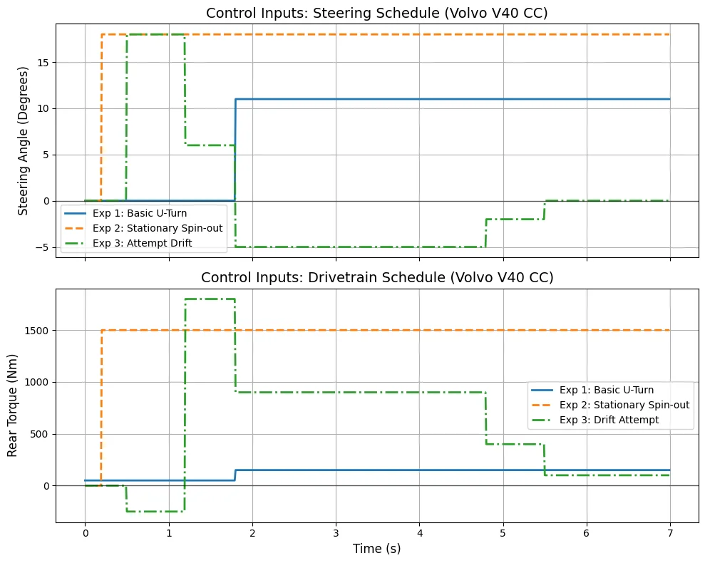
3. Scenario-based Experiments
We designed 3 scenarios:
- Basic U-Turn
- Stationary Spin-out
- Drift Attempt
Each scenarios is exactly 7 seconds long, again, at $dt = 0.01s$ Euler discretization.
The control graphs are as follow:
# Define the time vector for 7 seconds
dt = 0.01
t = np.arange(0, 7.0, dt)

# Initialize control arrays
delta1, T1 = np.zeros_like(t), np.zeros_like(t)
delta2, T2 = np.zeros_like(t), np.zeros_like(t)
delta3, T3 = np.zeros_like(t), np.zeros_like(t)

# Populate the schedules
for i, time in enumerate(t):

    # ---------------------------------------------------------
    # Experiment 1: Basic U-Turn
    # ---------------------------------------------------------
    if time < 1.8:
        delta1[i], T1[i] = 0.0, 50.0
    else:
        delta1[i], T1[i] = 11.0, 150.0

    # ---------------------------------------------------------
    # Experiment 2: Stationary Spin-out
    # ---------------------------------------------------------
    if time < 0.2:
        delta2[i], T2[i] = 0.0, 0.0
    else:
        delta2[i], T2[i] = 18.0, 1500.0

    # ---------------------------------------------------------
    # Experiment 3: Drift Attempt
    # ---------------------------------------------------------
    if time < 0.5:
        delta3[i], T3[i] = 0.0, 0.0
    elif time < 1.2:
        delta3[i], T3[i] = 18.0, -250.0
    elif time < 1.8:
        delta3[i], T3[i] = 6.0, 1800.0
    elif time < 4.8:
        delta3[i], T3[i] = -5.0, 900.0
    elif time < 5.5:
        delta3[i], T3[i] = -2.0, 400.0
    else:
        delta3[i], T3[i] = 0.0, 100.0

# --- Plotting ---
fig, (ax1, ax2) = plt.subplots(2, 1, figsize=(10, 8), sharex=True)

# Top Plot: Steering Angle
ax1.plot(t, delta1, label='Exp 1: Basic U-Turn', linewidth=2)
ax1.plot(t, delta2, label='Exp 2: Stationary Spin-out', linewidth=2, linestyle='--')
ax1.plot(t, delta3, label='Exp 3: Attempt Drift', linewidth=2, linestyle='-.')
ax1.set_ylabel("Steering Angle (Degrees)", fontsize=12)
ax1.set_title("Control Inputs: Steering Schedule (Volvo V40 CC)", fontsize=14)
ax1.axhline(0, color='black', linewidth=1, alpha=0.5)
ax1.grid(True)
ax1.legend()

# Bottom Plot: Rear Torque
ax2.plot(t, T1, label='Exp 1: Basic U-Turn', linewidth=2)
ax2.plot(t, T2, label='Exp 2: Stationary Spin-out', linewidth=2, linestyle='--')
ax2.plot(t, T3, label='Exp 3: Drift Attempt', linewidth=2, linestyle='-.')
ax2.set_xlabel("Time (s)", fontsize=12)
ax2.set_ylabel("Rear Torque (Nm)", fontsize=12)
ax2.set_title("Control Inputs: Drivetrain Schedule (Volvo V40 CC)", fontsize=14)
ax2.axhline(0, color='black', linewidth=1, alpha=0.5)
ax2.grid(True)
ax2.legend()

plt.tight_layout()
plt.show()
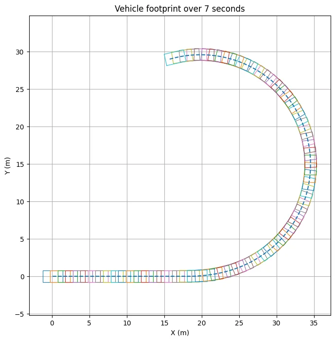
Additional plotting functions:
- Vehicle Footprint plot
# ...experiment code here

# --- plotting ---
plt.figure(figsize=(8, 8))

# vehicle dimensions
L = params.Lf + params.Lr
W = 2 * params.c

def draw_car(x, y, psi):
    corners = np.array([
        [ L/2,  W/2],
        [ L/2, -W/2],
        [-L/2, -W/2],
        [-L/2,  W/2],
        [ L/2,  W/2]
    ])

    R = np.array([
        [np.cos(psi), -np.sin(psi)],
        [np.sin(psi),  np.cos(psi)]
    ])

    rotated = corners @ R.T
    rotated[:, 0] += x
    rotated[:, 1] += y

    plt.plot(rotated[:, 0], rotated[:, 1], linewidth=0.8)

# draw every ~0.1s for clarity
for i, (x, y, psi) in enumerate(history):
    if i % 10 == 0:
        draw_car(x, y, psi)

# also plot path of center
xs = [h[0] for h in history]
ys = [h[1] for h in history]
plt.plot(xs, ys, linestyle='--')

plt.axis('equal')
plt.title("Vehicle footprint over 7 seconds")
plt.xlabel("X (m)")
plt.ylabel("Y (m)")
plt.grid(True)
plt.show()
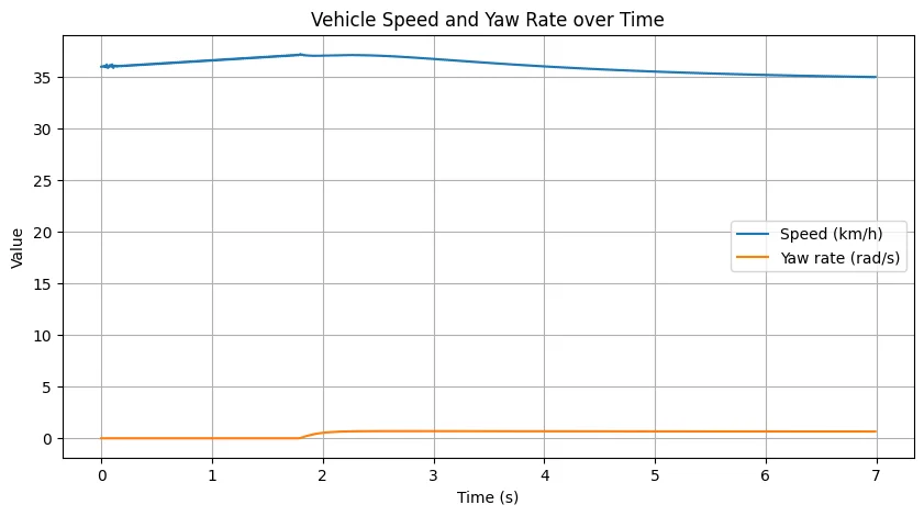
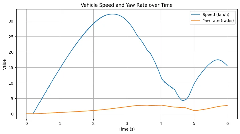
- Body’s Velocity vs Yaw Rate plot
plt.figure(figsize=(10, 5))

plt.plot(time_hist, vel_hist, label="Speed (km/h)")
plt.plot(time_hist, yaw_hist, label="Yaw rate (rad/s)")

plt.xlabel("Time (s)")
plt.ylabel("Value")
plt.title("Vehicle Speed and Yaw Rate over Time")
plt.grid(True)
plt.legend()

plt.show()
3.1. Basic U-Turn
T_total = 7.0
dt = params.dt
N = int(T_total / dt)

vel_hist = []
yaw_hist = []
time_hist = []

x, y, psi = 0.0, 0.0, 0.0

history = []

for i in range(N):
    t = i * dt

    if t < 1.8:
        delta = 0.0
        T = 50.0

    else:
        delta = np.deg2rad(11.0)
        T = 150.0

    control = ControlInput(delta=delta, T_rr=T, T_rl=T)

    state = model.step(state, control)

    vx, vy, r = state.vx, state.vy, state.r

    x += (vx * np.cos(psi) - vy * np.sin(psi)) * dt
    y += (vx * np.sin(psi) + vy * np.cos(psi)) * dt
    psi += r * dt

    v = np.sqrt(vx**2 + vy**2) * 3.6

    vel_hist.append(v)
    yaw_hist.append(r)
    time_hist.append(t)

    history.append((x, y, psi))
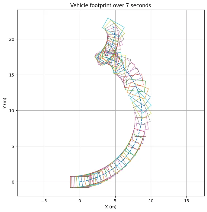
3.2. Stationary Spin-out
v0 = 0.0

state = VehicleState(
    vx=v0, vy=0.0, r=0.0,
    omega_fl=0.0, omega_fr=0.0,
    omega_rl=0.0, omega_rr=0.0
)

T_total = 6.0
dt = params.dt
N = int(T_total / dt)

vel_hist, yaw_hist, time_hist, history = [], [], [], []
x, y, psi = 0.0, 0.0, 0.0

for i in range(N):
    t = i * dt

    if t < 0.2:
        delta = 0.0
        T = 0.0

    else:
        delta = np.deg2rad(18.0)
        T = 1500.0

    control = ControlInput(delta=delta, T_rr=T, T_rl=T)
    state = model.step(state, control)

    vx, vy, r = state.vx, state.vy, state.r
    x += (vx * np.cos(psi) - vy * np.sin(psi)) * dt
    y += (vx * np.sin(psi) + vy * np.cos(psi)) * dt
    psi += r * dt

    vel_hist.append(np.sqrt(vx**2 + vy**2) * 3.6)
    yaw_hist.append(r)
    time_hist.append(t)
    history.append((x, y, psi))
3.3. Drift Attempt
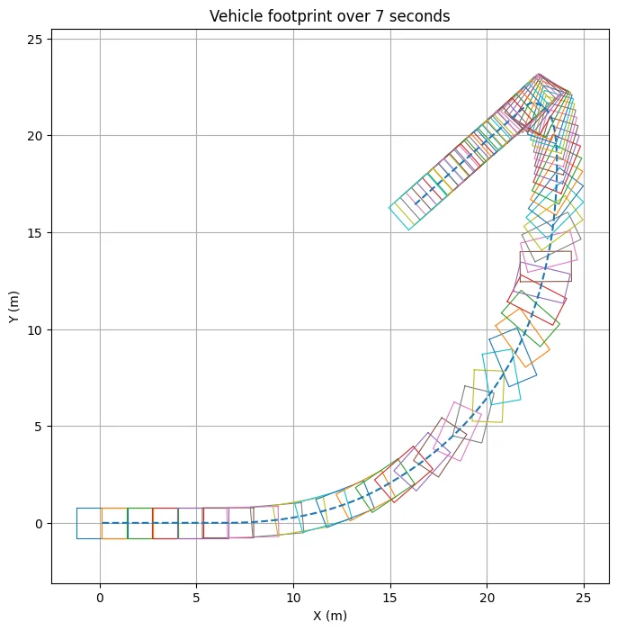
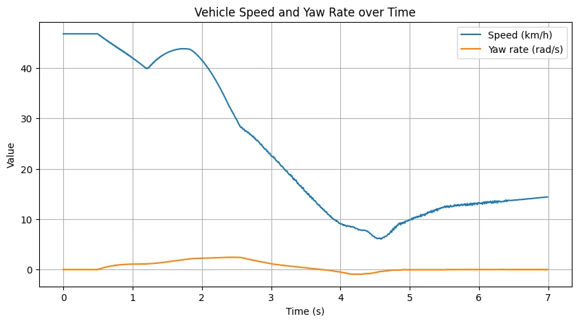
v0 = 13.0  # m/s (~47 km/h), slightly higher startoff speed

state = VehicleState(
    vx=v0, vy=0.0, r=0.0,
    omega_fl=v0 / params.R, omega_fr=v0 / params.R,
    omega_rl=v0 / params.R, omega_rr=v0 / params.R
)

T_total = 7.0
dt = params.dt
N = int(T_total / dt)

vel_hist, yaw_hist, time_hist, history = [], [], [], []
x, y, psi = 0.0, 0.0, 0.0

for i in range(N):
    t = i * dt

    if t < 0.5:
        delta = 0.0
        T = 0.0

    elif t < 1.2:
        delta = np.deg2rad(18.0)
        T = -250.0

    elif t < 1.8:
        delta = np.deg2rad(6.0)
        T = 1800.0

    elif t < 4.8:
        delta = -np.deg2rad(5.0)
        T = 900.0

    elif t < 5.5:
        delta = -np.deg2rad(2.0)
        T = 400.0

    else:
        delta = 0.0
        T = 100.0

    control = ControlInput(delta=delta, T_rr=T, T_rl=T)
    state = model.step(state, control)

    vx, vy, r = state.vx, state.vy, state.r
    x += (vx * np.cos(psi) - vy * np.sin(psi)) * dt
    y += (vx * np.sin(psi) + vy * np.cos(psi)) * dt
    psi += r * dt

    vel_hist.append(np.sqrt(vx**2 + vy**2) * 3.6)
    yaw_hist.append(r)
    time_hist.append(t)
    history.append((x, y, psi))
4. Attempts to Reproduce Results with Assetto Corsa
Now again, I’m just trying to do what I can, we don’t have access to professional proprietary software, nor can we easily inject scheduled controls into Assetto Corsa or extract its telemetry directly. Because of that, below is a video of me trying my best to recreate the scenarios using a similar car in parameters: The BMW M3 E92.
Since this is purely qualitative, I’ll let you decide the results.
5. Conclusion
Ultimately, these derivations and experiments lead to a necessary realization: vehicle dynamics models are mathematical approximations, not exact digital twins. Even when following a rigorous PhD-level framework, significant discrepancies between the model and real-world behavior (or high-fidelity simulators) are unavoidable.
The Reality of Modeling Constraints
- Dimensional Limitations: The 7-state planar model is a high-level abstraction. By focusing on the $XY$ plane, it inherently ignores vertical dynamics, pitch, and roll. In a real vehicle, the way a car “dives” under braking or “squats” under acceleration changes the tire contact patch in ways a 2D model cannot fully capture.
- Empirical vs. Physical Data: Formulas like the Pacejka Magic Formula are empirical curve-fits. They describe what happens to a tire under specific test conditions, but they don’t simulate the underlying molecular physics of rubber, temperature fluctuations, or road surface irregularities.
- System Complexity: Professional tools like CarSim succeed not just because of better math, but because they account for hundreds of additional variables, such as suspension bushing compliance, steering rack flex, and aerodynamic lift, that are simplified or omitted in standalone scripts.
Epilogue
It is worth noting that even the primary reference for this derivation acknowledged that their model could not perfectly match the behavior of industry-standard simulators. This doesn’t invalidate the model; rather, it defines its purpose. These equations are designed to provide a qualitative framework for understanding vehicle behavior and control logic, but they cannot realistically account for every nuance of physical vehicle dynamics.