Hybrid A*: A Path-planning Algorithm for Self-Driving Cars
Table of Content
Block
Prologue
I mean need I say more, I already recently learned about vehicle models, and I got a DAA course this semes too (idk what its short for tbh, algorithms or smt). Well, to be honest this project isn’t that suited for the final project assignment, its probably too many algorithms for what they ask for (I guess they want like, analyze 1 or few algo deeply in both space and complexity, name drop greedy, DP, and P vs. NP and that stuff), but I don’t care, I’m did this anyway, I do believe this project - Hybrid A* Playground is a major milestone in my journey for my new Autonomous Vehicles / Simulation niche.
- Github Repo: duy-phamduc68/Hybrid-A-Star-Playground
In a nutshell, Hybrid A* is a path-planning algorithm for self-driving car, that’s about as simple as I can put it. What I’m gonna do in this post, is go through the making process of this project at a high level, I think this is one of those project that is complex but also very doable in a reasonable amount of time, and what you can learn from it is paramount.
This project was inspired greatly by Practical Search Techniques in Path Planning for Autonomous Driving from Stanford.
1. Holonomic vs. Non-holonomic Robots
Alright so, self-driving car is actually a type of robot if you think about it, I mean if you’re a CS student, then you shrink an AV down to a RC car, maybe remove one of it axis leaving only 2 wheels, and I’m sure you’re going to call it a robot. So anyway, path-planning is one of the cornerstone of the robotics field.
But then maybe you’re wondering, then why don’t I say “Hybrid A* is a path-planning algorithm for robots” instead? Well it would still be technically true, but that wouldn’t highlight the nature of Hybrid A* as explicitly, that is, Hybrid A* is designed for Non-Holonomic Robots.
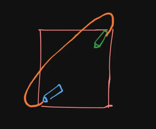
In robotics we usually have 2 types of robots that can be classified as Holonomic Robots and Non-Holonomic Robots. Their formal definition comes from Mechanics, and there’s a bunch of rigorous framework around how a robot is classified here, but for the scope of this post, I’m just gonna put this one drawing to explain how a self-driving car is a non-holonomic robot:
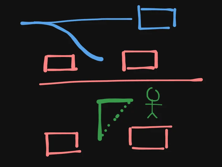
As you can see, in the top scenario, this is what we have, a car, in a parallel parking scenario, you can see the path that it would most likely have to take to park in between those 2 cars.
In the bottom scenario, we have a human (if you want to compare machine-to-machine, then imagine it a humanoid robot lol) and the path to the same position is much more straightforward, either a L shaped path or the dashed-diagonal will allow the human to reach the same position that took the car the entire parallel parking maneuver.
And if we strictly consider movement in a flat plane (both a human and a car can’t fly - yet), then the car here will be considered Non-Holonomic, while the human is Holonomic.
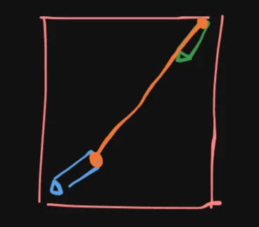
Consider this example:
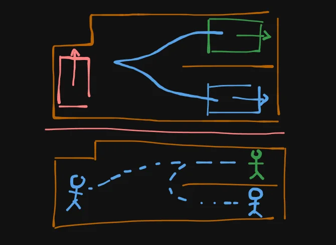
In the top scenario, the blue car can reach the green position, but the red car cannot. While in the bottom scenario, its not just that both human can reach the green position, but a human at any starting point can reach the green position if you think about it.
Now you can imagine that if we were in a 2D grid, and we think about the human / humanoid robot as an agent that can move in 8 directions, then that would be a holonomic robot, and normal A* will work just fine for it, I found this wonderful video that can help you Dijkstra and A* on a grid if you have never seen it before:
If we now replace the humanoid robot with a car, it obviously cannot move in 8 direction like the example above, not to mention, it also doesn’t just “jump a tile”, instead, it moves continuously in the physical world, and this core distinction is what Hybrid A* is all about.
There is definitely better and more rigorous explanation for this, but this was what got me through it…
2. Kinematic Bicycle Model
Although I’ve already learned about this, I think its better to just show you, use the custom simulator below to just understand what a Kinematic Bicycle Model is intuitively (sorry mobile user):
KINEMATIC BICYCLE
Alright text time, we simplify a car with 4 wheels into a bicycle with 2 wheels, why? Simplicity, its extremely easy to implement and simulate instead of a full physics engine, so a lot of robotics algorithm, especially early autonomous vehicles work, was built under the assumption that the car is a Kinematic Bicycle Model. This was the model I used in the project.
2.1. Formal Definition (Differential Equations)
The model assumes the rear wheel is fixed to the frame and the front wheel steers. In the simulation, the red wheel (rear) always follows the body heading $\theta$, while the blue wheel (front) is offset by the steering angle $\delta$.
The differential equations for the state $(x, y, \theta)$ are:
Block
- $v$: The velocity (the V value on your display).
- $L$: The wheelbase (the length of the white line connecting the wheels).
- $\theta$: The direction the chassis is pointing.
You control this car with $(v, \delta)$. Specifically, if you have 2 analog controls, say $u$ that has range 0.0 to 1.0 and $s$ that has range -1.0 to 1.0, then:
Block
When you steer, the vehicle rotates around an imaginary point called the Instantaneous Center of Rotation (ICR). This is the center of the faint gray circle that appears in the simulation.
The radius $R$ of that circle is calculated as:
Block
The gray dashed arc is just a preview of the turning circle’s circumference. Since the change in heading ($\dot{\theta}$) is simply velocity divided by radius:
Block
- Tight Turns: A larger $\delta$ makes $\tan(\delta)$ bigger, which makes $R$ smaller (a tighter gray circle).
- Straight Lines: When $\delta$ is $0$, the radius $R$ becomes infinite, the gray circle disappears, and $\dot{\theta}$ becomes $0$, perfectly straight travel.
2.2. Integration & Code
Since computers can’t calculate continuous motion, we use Euler Integration. We take a tiny slice of time ($dt$) and assume the velocity and steering stay constant during that slice.
2.2.1. Discretized Formulas
For every frame in the simulation, we update the state like this:
Block
2.2.2. Minimal Python Implementation
import math

# Params

# Wheelbase
L = 50.0
# Top speed (if L = 50.0 is 5m, then MAX_V is 15m/s)
MAX_V = 150.0
# Max steering angle (radian, ~= 40 degrees)
MAX_STEER = 0.7
# 0.2s ramp-up
RAMP = 0.2
# 60Hz tick / 60FPS
dt = 0.016

# State
x, y, theta = 0.0, 0.0, 0.0
v = 0.0
delta = 0.0

def update_sim(keys):
    global x, y, theta, v, delta

    # 1. Process Velocity Input (W/S)
    accel = MAX_V / RAMP
    if 'w' in keys:
        v = min(v + accel * dt, MAX_V)
    elif 's' in keys:
        v = max(v - accel * dt, -MAX_V)
    else:
        v *= 0.9  # Quick friction decay

    # 2. Process Steer Input (A/D)
    if 'a' in keys:
        delta = max(delta - 0.1, -MAX_STEER)
    elif 'd' in keys:
        delta = min(delta + 0.1, MAX_STEER)
    else:
        delta *= 0.8  # Auto-center decay

    # 3. Kinematic Integration
    x += v * math.cos(theta) * dt
    y += v * math.sin(theta) * dt
    theta += (v / L) * math.tan(delta) * dt

# Example usage: simulate holding 'W' and 'D'
active_keys = ['w', 'd']
for _ in range(100):  # Equal to 1.6 seconds of simulated time
    update_sim(active_keys)
    print(f"V: {v:.1f}")
    print(f"Steer: {math.degrees(delta):.1f}")
    print(f"Pos: ({x:.1f}, {y:.1f})")
3. The A* Algorithm
Now, I assume you are already familiar with the Dijkstra algorithm, if not, you should go watch some videos about it, because A* is basically Dijkstra++. If recommend this video:
And to compare Dijkstra and A* again (and other search algorithms):
(The video above, the agent seems to only be able to move in 4 directions, in our own code and implementation we are going to use 8 directions for consistency)
After watching the examples, we can checkout the following code:
import heapq
import math

def dijkstra_grid_8(grid, start, goal):
    rows, cols = len(grid), len(grid[0])
    pq = [(0, start)]
    distances = {start: 0}
    came_from = {}

    while pq:
        curr_dist, (r, c) = heapq.heappop(pq)

        if (r, c) == goal:
            path = []
            while (r, c) in came_from:
                path.append((r, c))
                (r, c) = came_from[(r, c)]
            path.append(start)
            return path[::-1]

        for dr, dc in [(0,1),(0,-1),(1,0),(-1,0),(1,1),(1,-1),(-1,1),(-1,-1)]:
            nr, nc = r + dr, c + dc
            if 0 <= nr < rows and 0 <= nc < cols and grid[nr][nc] == 0:
                weight = math.sqrt(dr**2 + dc**2)
                new_dist = curr_dist + weight
                if new_dist < distances.get((nr, nc), float('inf')):
                    distances[(nr, nc)] = new_dist
                    came_from[(nr, nc)] = (r, c)
                    heapq.heappush(pq, (new_dist, (nr, nc)))
    return None
import heapq
import math

def a_star_grid_8(grid, start, goal):
    rows, cols = len(grid), len(grid[0])

    def heuristic(a, b):
        return math.sqrt((a[0] - b[0])**2 + (a[1] - b[1])**2)

    pq = [(heuristic(start, goal), 0, start)]
    g_score = {start: 0}
    came_from = {}

    while pq:
        f, g, (r, c) = heapq.heappop(pq)

        if (r, c) == goal:
            path = []
            while (r, c) in came_from:
                path.append((r, c))
                (r, c) = came_from[(r, c)]
            path.append(start)
            return path[::-1]

        for dr, dc in [(0,1),(0,-1),(1,0),(-1,0),(1,1),(1,-1),(-1,1),(-1,-1)]:
            nr, nc = r + dr, c + dc
            if 0 <= nr < rows and 0 <= nc < cols and grid[nr][nc] == 0:
                weight = math.sqrt(dr**2 + dc**2)
                tentative_g = g + weight
                if tentative_g < g_score.get((nr, nc), float('inf')):
                    came_from[(nr, nc)] = (r, c)
                    g_score[(nr, nc)] = tentative_g
                    f_score = tentative_g + heuristic((nr, nc), goal)
                    heapq.heappush(pq, (f_score, tentative_g, (nr, nc)))
    return None
As you can see, A* is basically Dijkstra + Heuristic. The difference between them can best be felt in environments more specific than the default graph where these algorithms is usually taught (you can decompose search space in different environments into graphs anyway).
In our case, where the environment is a 2D grid, you can see that A* has a sense of “direction” when searching in such a space, usually, this is thanks to a Euclidean distance heuristic like the code above.
When A* searches, imagine that at any tile, it doesn’t just only know how far it has gone (like Dijkstra), but also how relatively close it is to the goal in this particular case. Its kinda like the agent has wallhacks basically:
While Dijkstra is guaranteed to find the shortest path, it wastes a lot of time exploring areas that are obviously moving away from the goal. By adding the heuristic, A* significantly reduces the number of nodes it needs to check.
What I want you to focus on first, is the Cost Function:
Block
Here, $g(n)$ is the accumulated cost (G-Cost), it helps determining which path is more preferable, in Dijkstra only $g(n)$ exists implicitly in the priority queue, while in A-star, we also have the heuristic cost (H-Cost) $h(n)$. And A-star’s priority queue evaluates $f(n)$ - the cost function.
4. The Search Space of Hybrid A*
Before we get into the Cost Function though, we must understand what kind of search space are we working in.
Let’s bring our last 2 sections together, a Continuous, Non-holonomic Kinematic Bicycle Model inside of a 2D Grid where A* can operate on with a Holonomic agent, yeah, there’s definitely a mismatch here.
Remember in 2.2.1. Discretized Formulas where we did indeed confirm that the continuous model still has to be represented and simulated in discrete timestep, but then again, for very low timestep like 0.001s, which is often the case for vehicle model in autonomous driving stack because we need to be accurate in such a high stake task, then if we consider each state to be a tile or a node in the search space, then it can often explode to the millions.
A car position isn’t just (int, int) like (0, 0) or (2, 0), they are (float, float).
Even if 2 state of a car end up in the same position on the grid, its orientation can span 360 degrees, and can be fractional! (we often store degrees as radian and convert for easy floating point operations).
And this is where the “Hybrid” in Hybrid A* comes from, that is, our agent, our states, is continuous, but the search is still done in discrete space. Think about it like this:
Let’s just say that technically our grid is continuous, even though we place walls that snap to grid for simplicity but they are still considered continuous, especially with respect to the car, then if we just draw it out our environment would look something like this:
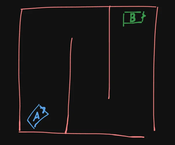
Where the A car is the start, and B car is the goal.
And, this is how we are going to Discretize the Search Space:
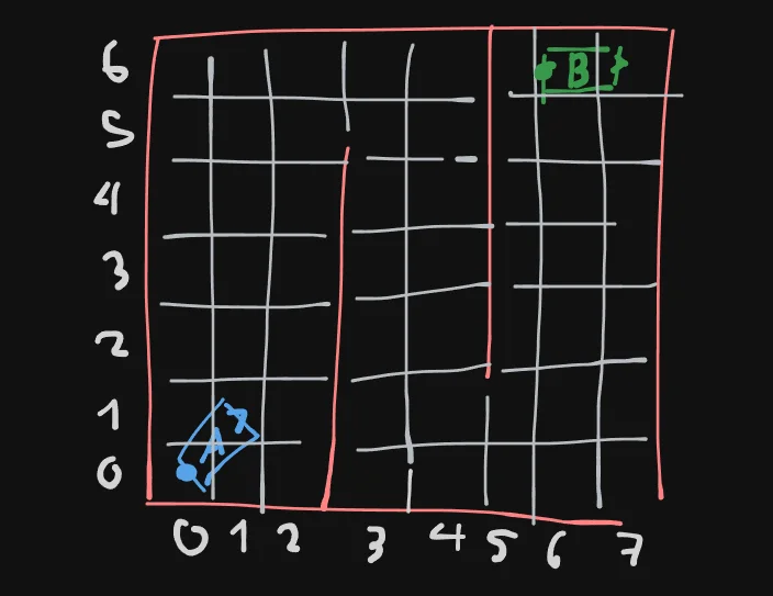
Yeah, we… still use grids, and remember that the $x, y$ state is defined at the rear axle of the car, so I’ve added dots to highlight them, now, you can imagine how these dots are assigned to their grid tile now, so, the A car will be treated as if its in tile (0, 0), and the B car in tile (6, 6). And for the obstacles / walls… well, i didn’t really thought this through… but how about this:
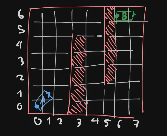
Now, the obstacles take up:
[(3, 0), (3, 1), (3, 2), (3, 3), (3, 4)]

and

[(5, 2), (5, 3), (5, 4), (5, 5), (5, 6)]
And, if we stop here, yeah its just normal A* now, a start, a goal, obstacles, in a discrete 2D grid, all with nice 2 int tuples (int, int). Might be looking like going in circles, but now, here’s the kicker, we don’t stop here, we don’t just stop at discretizing the search space into a 2D grid, because the next step, is also discretizing the heading of the car, so now, imagine that each grid tile can finally represent a state of our bicycle model: $(x, y, \theta)$. That tuple have 3 numbers, what does that make you think of? A 3D grid:
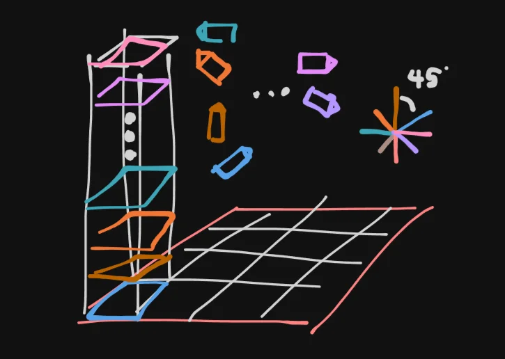
For simplicity sake, lets discretize our heading bins for each tile into 8 direction, each 45 degrees from eachother, and you have this mental model above.
So now, we can clearly classify the A and B car into: (0, 0, 1) and (6, 6, 0) (assuming same direction as the Unit Circle).
So if we come back to A* now, technically, we can use still use these 3D states for searching, we apply the Euclidean heuristic to the first 2 values which is x, y, and then we just do a for loop to check for all 8 heading bins and yeah we can technically go from (0, 0, 1) to (6, 6, 0) like this, but what I really want you to grasp here is the way Hybrid A* Discretize the Search Space into a 3D grid.
Moreover, if we discretize at increasingly higher fidelity, so say if we didn’t just made it into a 6 x 7 but 60 x 70 or even 600 x 700 grid, and the heading bins, instead of 8 direction, maybe 360 / 5 = 72, then you can imagine how it can greatly improve how these discretized grid can tell us how close we are to a state.
In this case, 60 x 70 x 72 = 302,400 possible discrete states, but here’s the thing, we don’t exactly search in this space as if we are running for-loops for each of the states, its more about keeping track of where and how the car has reached somewhere.
Not to mention, now lets say if we have 2 car state: (0.75, 1.99, 45.4) and (0.75, 2.01, 44.9), then they both will be rounded off and assigned to bin (1, 2, 1), which again significantly shrink the search space.
So, lets just stick with this configuration through out, whenever I draw a board like
again, just imagine that under the hood, its a 3D grid of 60 x 70 x 72 = 302,400 cubes / nodes.
5. Heuristic (H-Cost) of Hybrid A*
5.1. How the Car moves in the environment
Now, the car still need a way to reach a state somehow in our grid, take a look at the real-axle defined kinematic bicycle model again, what I want you to think about is Motion Primitives, while the maximum “reach” of the car is dependant on a lot of factor such as MAX_V, MAX_STEER, dt, etc… its “actions” will always be 6 for a car that has a reverse gear:
straight
left
right
reverse
reverse-left
reverse-right
Visually, it kinda looks like a spider:
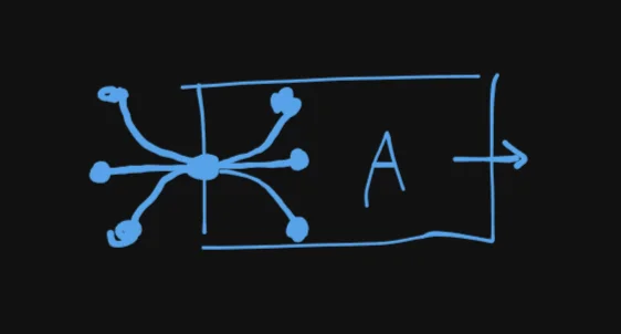
In the image above, each of the dots here can be considered a node, this is a bit confusing if we already call the 3D grid in section 4 nodes, so let define the nodes belonging to the 3D grid discrete nodes, and these nodes representing car states continuous nodes, which mean that continuous nodes are assigned to discrete nodes.
So, if in the normal A* example the agent can move in 8 directions and thus at any step can have 8 actions, and can reach 8 other discrete nodes assuming no collision occurs, then for our car, at any step the amount of actions, ie. motion primitives it can take and the amount of discrete nodes it can reach is not always a constant even if there is no obstacles.
If we have a 3D grid with high-fidelity, and we accept some buffer space for what we consider “reaching the goal” for now, then the goal can be reached when our car reach a certain discrete node, this is when we are going to have to rethink about the heuristic.
Once the car reached this goal in a discrete node, its going to have to reconstruct its exact maneuvers by backtracking its continuous nodes.
5.2. Examples to Explain the Heuristic
Okay so, earlier I was joking when I said we can do normal A* by still using Euclidean and just looping through to see which heading match. The fact is, for Hybrid A* we need to use a very specific heuristic function that is also kinda hybrid in of itself, in short:
Block
yeah I’m just gonna name drop it there, don’t worry about it too much for now, to really grasp it, I’m going to give some examples.
5.2.1. The H2D Heuristic
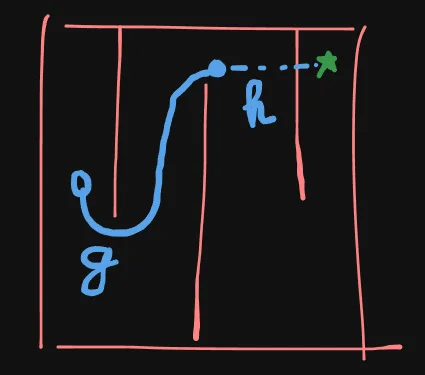
I’d like to call $h_{H2D}$ the “obstacle-knowing, physics-ignoring” heuristic. Consider the following examples:
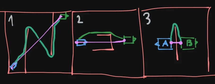
Here, the pink line represent the euclidean distance ignoring obstacles just like normal A, while the teal line… its like running A… but the key here is that we run it already before we even enter the main loop of Hybrid A, so as you can see by running A first like this, we will know:
- Roughly where the obstacles are (example 1)
- If there are any deadends (example 2)
- And sometimes can help in cases where start and goal is deceivingly close (example 3)
We know all of this with out having to straight up drive the non-holonomic car. Which also make it ignore the physics of the car, it will know a tiny test tube shaped obstacle is a deadend, regardless of whether or not the car can even fit in there.
And here’s the thing, H2D is also special in that we can pre-compute it, we don’t even have to run it or update it during the main loop of Hybrid A* itself given a static environment. Fact is if we use the goal as the source of a Dijkstra, then we use it to compute the distance from the goal discrete node to every other discrete nodes, then we will basically have a $O(1)$ look up grid for H2D.
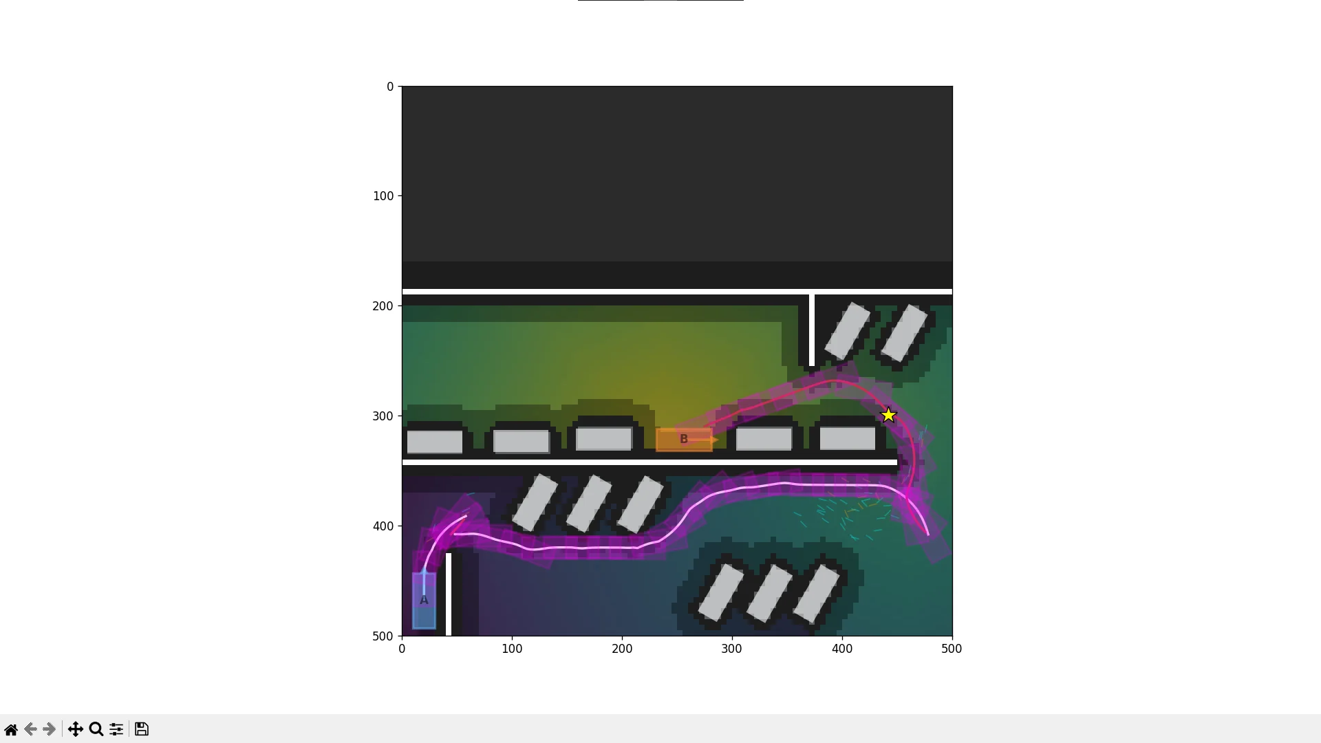
So, beside from “obstacle-knowing, physics-ignoring”, $h_{H2D}$ is also pre-computed. Below is an image to help you get the idea better:

Here, you can see the gradients in the background represent $h_{H2D}$ note how the obstacles (black and white pixels) clearly affect H2D, and that purple part is obviously a deadend.
More importantly, in the example above (it says 500 x 500 but thats pixels, the size of this grid is 100 x 100), $h_{H2D}$, which is pre-computed by this goal-origin Dijkstra is only ran on the 100 x 100 = 10,000 2D grid which is still in a reasonable range for Dijkstra, so each of those tiles will know “how far it is from the goal”, notice that we do not include the heading bins in this heuristic, we will comeback to this.
5.2.2. The Analytical Heuristic
This part is a bit more complex, or perhaps, more alien to those who come from a CS background, in this section, I’m gonna briefly cover Dubins and Reeds Shepp path, which is our “obstacle-ignoring, physics-respecting” heuristic, mostly about how it matters to our pipeline so far, because honestly, others explain it way better than me. These two videos from Aaron Becker was especially helpful:
What I really want you to take away from these videos are:
- Explain to a 10 yo: Dubins is a plane (forward only, ie. 3 motion primitives); Reeds-Shepp is a car (can reverse, ie. 6 motion primitives).
- Optimal & Closed-Form: Mathematical formulas that give the “perfect” shortest path in $O(1)$ time without searching, but ignores obstacles.
- The “Sniper-shot”: Used as an “Analytic Expansion” to snap directly to the goal when near it, bypassing the grid search, a sort of “sniper-shot”.
- The Heading Hack: By using the DB/RS distance as a heuristic, you capture the heading ($\theta$) constraint in real-time.
- H2D Independence: Because DB/RS handles the 3D $(x, y, \theta)$ physics, your precomputed $h_{H2D}$ only needs to focus on obstacles (Dijkstra). You don’t need to bloat your H2D table with heading data because the DB/RS component accounts for the turning radius.
For my project, I mostly use the Reeds Shepp path, thus, we have $h_{RS}$. Unlike H2D, this is not pre-computed.
5.3. Putting Together h(n)
Now, remember the name drop from Section 5.2.:
Block
You might be wondering, why are we using max here? Well, lets take a look:
500 x 500 pixels grid, thats like, technically the continuous space of the car here, just a very coarse one. On the diagonal, the length is ~ 700px = 500px * sqrt(2).
So, the longest length from the start to goal is 700px, and shortest is when start = goal, so for H2D:
0 <= h2d <= 700
For analytical cost, its a bit tricky, but remember that it ignores collision, even boundaries, so maybe a Dubins path’s worst case can be something like this:
So its probably roughly:
0 <= analytical_cost <= 1200
RS paths are never longer than Dubins for the same start/goal, Dubins paths is a subset of Reeds Shepp paths afterall. So if you actually if you imagine the above scenario with Reeds Shepp path (how to reach goal is literally just a straight reverse):
then you can imagine that actually in this case h2d ~= analytical_cost, so in other words, you can have the intuition that they describe the similar path under different simplifications. So if we were to say add them instead of taking the max, it would be saying:
Blockreal cost >= (distance ignoring yaw) + (distance ignoring obstacles)
Which as we see is not true, this will break a certain requirement of normal A* that is the admissibility of the heuristic, you probably can find somewhere that explains it more clearly but for this project its honestly not that important.
Just think of the 2 heuristic as 2 guides:
- Advisor A: “You need at least 700 units (distance)”
- Advisor B: “You need at least 715 units (turning constraints)”
You don’t say:
- “Okay, 1415 units”
You say:
- “At least 715”
5.4. Expanding h(n)
What’s cool about $h(n)$ in Hybrid A*, is that you can also add extra heuristic to satisfy certain requirements you may have, for example, in my implementation, I actually use:
h_cost = max(h2d, analytic_cost) + proximity
To also discourage the car from getting too close to obstacles and walls. Adding this does break admissibility though, might need to look deeper into that.
6. Accumulated Cost (G-Cost) in Hybrid A*
This is honestly really quick to cover, go back to our 500x500px grid example, our $g(n)$ is just the length the car has traveled so far:
In the case above:
g(n) ~= 700
Considering our scenarios usually include twist and turns, you can expect g(n) to be roughly in the range of 1500 - 3000.
What’s important though, is that in g(n) you can again add certain requirements, in my implementation, every step the car takes, the accumulation of $g(n)$ is:
step_g = abs(v * dt)
if reverse: *= penalty_reverse
if gear change: += penalty_gear_shift
step_g += abs(steer) * penalty_steer
So paths that have a bunch of reverse (IRL, cars hate going in reverse) will be discouraged:
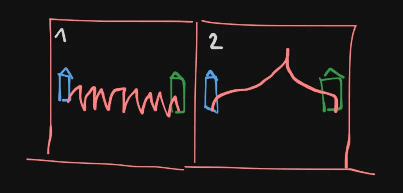
So my implementation will prefer example 2 even though technically example 1 will be considered “shorter” mostly by H2D.
What’s more, we can also prune paths early if $g(n)$ doesn’t improve by a certain threshold.
And thus, our cost function is finalized:
Block
By finding the path with the lowest Cost, in this particular implementation, we can understand intuitively that the path:
- Try not to go in reverse too much
- Respect kinematics / physics, while knowing where the obstacles are and how far it is to the goal
- Stay far from obstacles if possible
- Still shortest path within configuration
I might update a link for the Collision Engine for Hybrid A* post here.
7. Hybrid A* Main Loop
In my code implementation, its a bit mixed between rendering and the actual Hybrid A* logic, I will try to fix it soon, but here’s the gist of it:
open_set = []
visited_bins = {}
counter = 0

start_node = Node(...)
heapq.heappush(open_set, (0.0, counter, start_node))

while open_set:
    # 1. Pop best node (lowest f)
    _, _, current = heapq.heappop(open_set)

    # 2. Discretize (snap to bin)
    curr_key = (
        int(current.x // grid_size),
        int(current.y // grid_size),
        int(current.yaw // yaw_reso_deg),
    )

    # 3. Prune worse duplicates
    if curr_key in visited_bins:
        if current.g > visited_bins[curr_key] + tiny_epsilon:
            continue

    # 4. Goal check
    if near_goal(current):
        final_node = current
        break

    # 5. Try analytic shortcut (sniper)
    if within_sniper_radius(current):
        sniper = attempt_sniper(current)
        if sniper:
            final_node = sniper
            break

    # 6. Expand (THIS is the "hybrid" part)
    for direction in allowed_dirs:          # forward / reverse
        for steer_mul in steering_multipliers:  # left / straight / right

            steer = steer_mul * steer_max_deg
            v = v_max * direction

            # --- continuous simulation ---
            px, py, pyaw = kinematic_expansion(current, v, steer)

            nx, ny, nyaw = px[-1], py[-1], pyaw[-1]

            # 7. Collision check (along the arc)
            if samples_collide(px, py, pyaw):
                continue

            # 8. Snap new state to bin
            bin_key = (
                int(nx // grid_size),
                int(ny // grid_size),
                int(nyaw // yaw_reso_deg),
            )

            # 9. Compute g (actual cost)
            step_g = abs(v * dt)
            if direction == -1:
                step_g *= penalty_reverse
            if direction != current.direction:
                step_g += penalty_gear_shift
            step_g += abs(steer) * penalty_steer

            new_g = current.g + step_g

            # 10. Prune small improvements
            if bin_key in visited_bins:
                if (visited_bins[bin_key] - new_g) < min_g_improvement:
                    continue

            # 11. Heuristic (THIS is the "A*")
            h2d = h2d_grid[grid_y, grid_x]
            if h2d == inf:
                continue

            h = max(
                h2d * grid_size,
                analytic_cost(nx, ny, nyaw, goal)
            )

            h += obstacle_proximity_penalty(nx, ny, nyaw)

            # 12. Final cost
            f = new_g + h_cost_weight * h

            # 13. Record best g for this bin
            visited_bins[bin_key] = new_g

            # 14. Push new node
            counter += 1
            new_node = Node(
                nx, ny, nyaw,
                new_g, f,
                px, py, pyaw,
                [direction] * len(px),
                direction,
                current
            )

            heapq.heappush(open_set, (f, counter, new_node))
Lets ignore _samples_collide for now (check the note above Section 7.), and analyze this algorithmically.
7.1. Time Complexity
Block
Where:
-
$b$ (Branching Factor): In the code, this is
len(allowed_dirs) * len(steering_multipliers). (e.g., 2 directions $\times$ 3 steer angles = 6 for Reeds Shepp path). - $d$ (Depth): The number of “steps” (moves of length $v \cdot dt$) to reach the goal.
-
$K$ (The “Kinematic Tax”): In standard A*, moving to a neighbor is $O(1)$. In the code, each expansion involves:
-
kinematic_expansion: Simulating the arc. Usually $O(K)$. -
analytic_cost: Calculating Dubins/RS distance. Usually $O(1)$. -
samples_collide: Checking every point along that arc against the map. The bulk of $K$’s time complexity, but again, we don’t cover it in this post.
-
- Heuristic Impact: Because we are using Dual Heuristic ($\max(h_{H2D}, h_{RS})$), the “Effective Branching Factor” is much lower than $b$ because the search is highly directional toward the goal, pruning vast amounts of the state space.
7.2. Space Complexity
Block
The memory usage is dominated by how many states we store.
-
visited_bins: This is the primary memory consumer. The maximum size is proportional to the number of discrete “buckets” in our map (width * height * (360 / yaw_reso). -
open_set: In the worst case, the Priority Queue can grow to hold a significant fraction of these bins. -
Node Data: Each
Nodeobject in the code stores the entire path segment (px, py, pyaw). This makes the space complexity “heavy” compared to standard A* which only stores a parent pointer.
# hybrid_a_star/core/node.py

from __future__ import annotations

from dataclasses import dataclass
from typing import Optional

@dataclass
class Node:
    x: float
    y: float
    yaw: float
    g: float
    f: float
    path_x: list[float]
    path_y: list[float]
    path_yaw: list[float]
    path_dir: list[int]
    direction: int
    parent: Optional["Node"]
7.3. Key Constraints to Mention
7.3.1. Resolution Completeness
Hybrid A* is not “Complete” (it might fail to find a path even if one exists if our configuration, eg. grid_size or yaw_reso is too coarse). It is Resolution Complete, meaning it is guaranteed to find a solution given a fine enough discretization.
7.3.2. The “Sniper-shot” Efficiency
Algorithmically, the attempt_sniper (Dubins/RS) check is $O(1)$ time, but it drastically reduces the Average Time Complexity. By finding the “mathematical finish line” early, it prevents the $b^d$ exponential growth from reaching its full potential.
7.3.3. H2D Pre-computation
Don’t forget that our h2d_grid is pre-computed (Step 11), that adds a one-time $O(W \cdot H)$ Dijkstra cost before the main loop even starts.
I might update a link for the Smoothing Hybrid A* Paths with Gradient Descent here.
8. Hybrid A* Playground
- Github Repo: duy-phamduc68/Hybrid-A-Star-Playground
Some images:
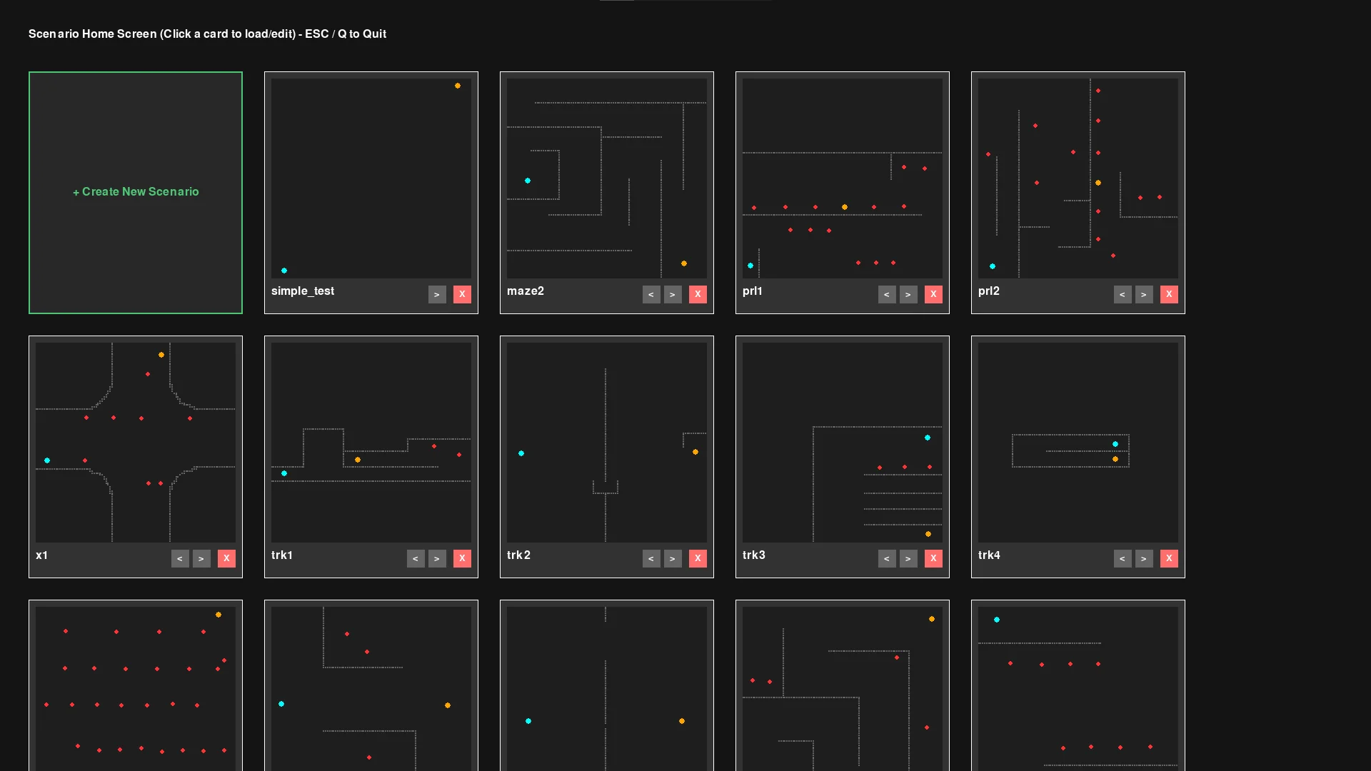
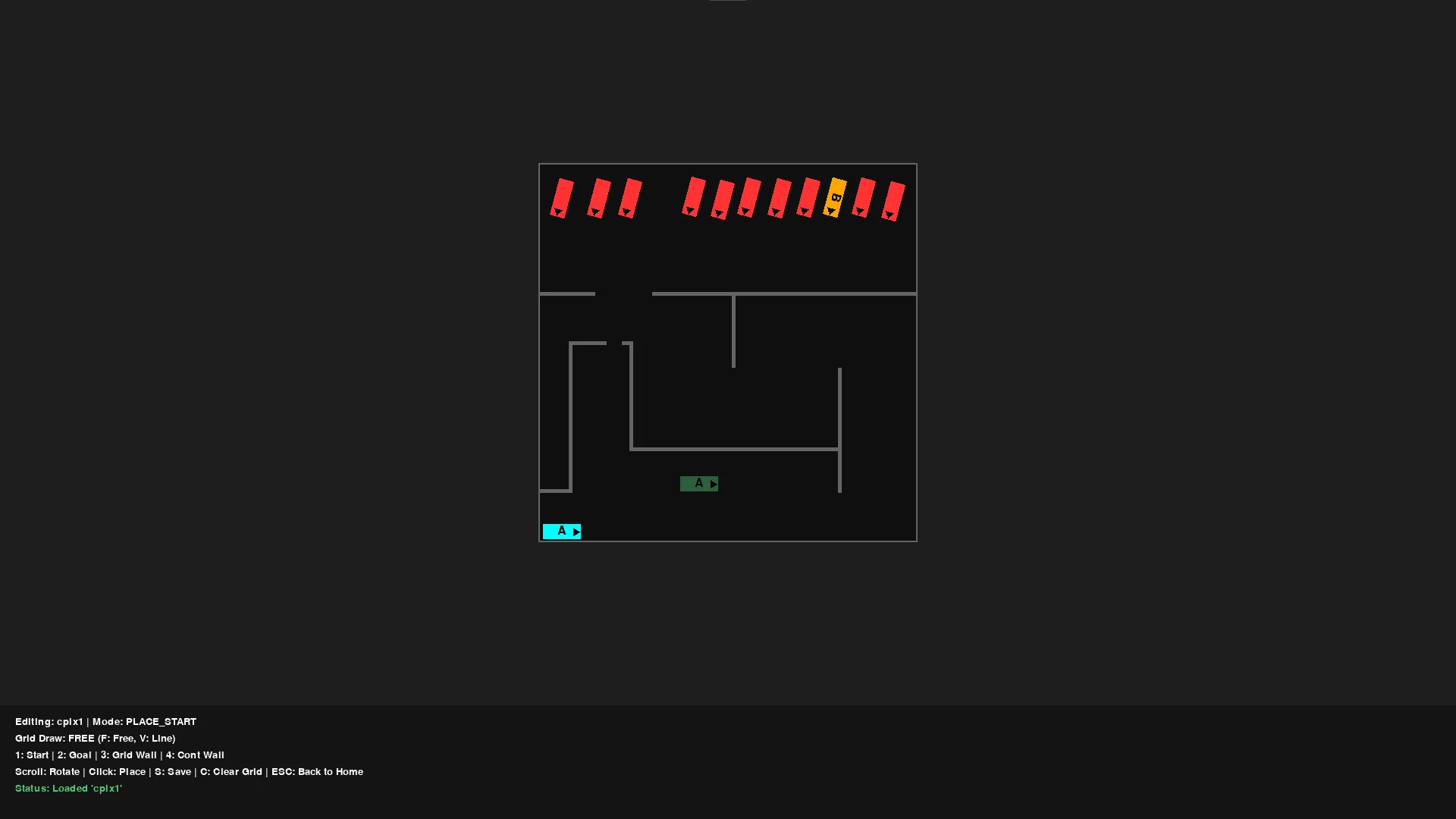
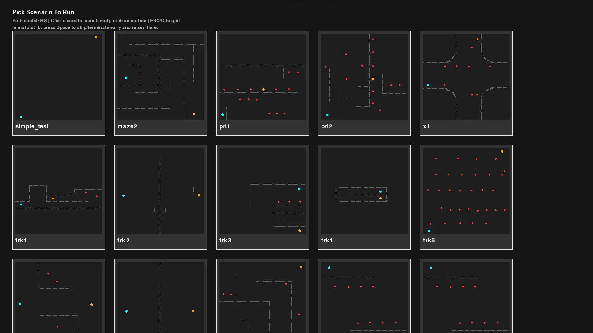
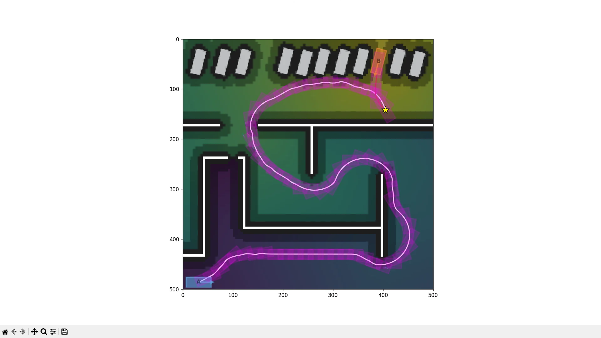
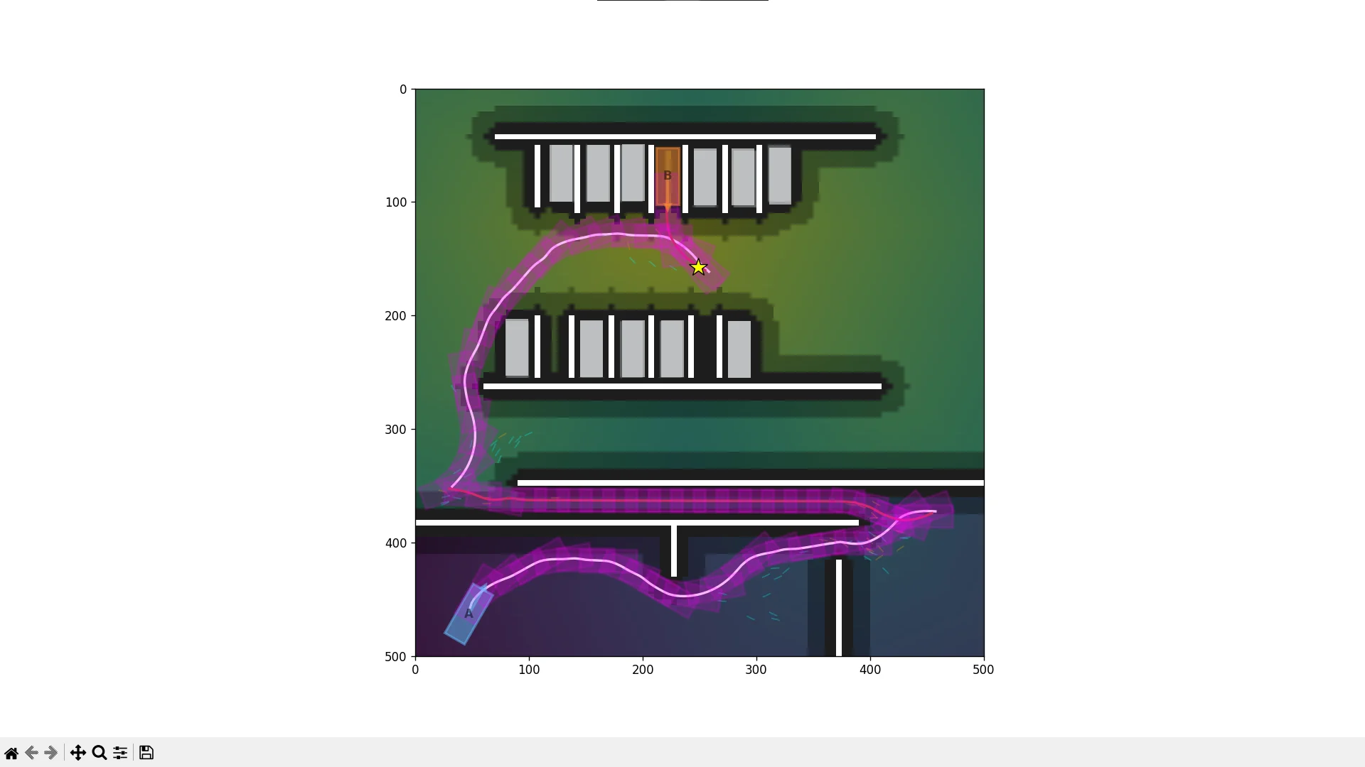
9. Limitations & Future Work
Right now, my implementation still take quite a while if the configuration is favorable, I’ve tweaked the default config to be relatively fast and fun to watch, but that also mean that, it could definitely miss a feasible path, and struggle in tight spaces.
For future work, maybe I will continue to work towards the inspiration for the project, the Stanford paper:
So that would most likely mean:
- The maze is not known ahead of time -> ray-casting collision detection, simulating an autonomous vehicle with sensors like LiDAR
- Avoid dynamic obstacles, so, other cars on the road
- A fancy 3D visualization lol
There is definitely more improvements and optimization I can give it, but for now, I’m quite happy with what I was able to learn from this project. For now, its time to write up the collision post and gradient descent post…