Table of Content

• Table of Content
• Roadmap
• Model 7 Recap
• 1. A Different Kind of Post in this Series
• 2. Freeze Frame: Reading the Diagram
• 2.1. What We’re Looking At
• 2.2. The Two Angles We Need to Internalize
• 2.3. Reading the Diagram Label by Label
• 2.4. About Simulator 6’s Predicted Trajectory
• 3. From Geometry to Forces: The Linear Tire Model
• 4. Promoting Yaw Rate to a State
• 4.1. The Mirror Table
• 4.2. Where Does Yaw Rate Come From
• 4.3. Deriving the Yaw Torque
• 5. The Full ODE System
• 5.1. The States
• 5.2. Computing Slip Angles
• 5.3. The ODE System
• 5.4. The Cheat That Survives into Model 7
• 6. Final Takeaways
• 7. Simulator 7 Showcase
• Epilogue

Block

• Main reference: Marco Monster’s Car Physics
• Github repo for Longitudinal Simulators: duy-phamduc68/Longitudinal-Car-Physics
• Github repo for Simulator 6: duy-phamduc68/Planar-Kinematic-Car-Model
• Github repo for Planar Dynamic Simulator(s): duy-phamduc68/Planar-Dynamic-Car-Model

Roadmap

• Model 1: Longitudinal Point Mass (1D)
  • Straight Line Physics
  • Magic Constants
  • Braking
• Model 2: Load Transfer Without Traction Limits (1D)
  • Weight Transfer
• Model 3: Engine Torque + Gearing without Slip (1D)
  • Engine Force
  • Gear Ratios
  • Drive Wheel Acceleration (simplified)
• Model 4: Wheel Rotational Dynamics (1D)
  • Drive Wheel Acceleration (full)
  • Torque on the Drive Wheel & The Chicken and The Egg
• Model 5: Slip Ratio + Traction Curve (1D)
  • Slip Ratio & Traction Force
• Model 6: Low-Speed Kinematic Turning (2D)
  • Curves (low speed)
• Model 7: High-Speed Lateral Tire Model (2D)
  • High Speed Turning
• Model 8: Full Coupled Tire Model (2D)

Block

Model 7 Recap

Model 7 is the lateral mirror of everything we built in Models 3-5, but applied to the car’s rotational and sideways motion. So:

• Like slip ratio driving forward traction, we now have slip angles driving lateral (cornering) forces
• Like having rotational wheel spin inertia ($d \omega / dt$), we now have yaw inertia ($dr / dt$)
• And like removing the “suction cup wheels” hack from Model 3-4, we now retire the “geometry dictates motion” hack from Model 6

The car can finally diverge from its heading. The velocity vector and the car body can point in different directions. That’s when we get sideslip, understeer, oversteer, drift,…

1. A Different Kind of Post in this Series

If you’ve been reading from Model 1, you’re probably used to a certain rhythm in these posts. We identify a new physical phenomenon, derive the force or torque it produces, write the ODE, then implement it. Models 1-6 followed that flow pretty cleanly because each model was introducing essentially one new concept at a time. Even with Model 6 when we thought going from 1D to 2D would be a big deal, but honestly going to Model 6 was more like lifting Model 5 on to a pivot rail.

Model 7 broke that pattern for me.

The problem is that Model 7’s new concepts: sideslip angle ($\beta$), slip angles ($\alpha_f, \alpha_r$), lateral tire forces ($F_{yf}, F_{yr}$), and yaw inertia ($I_z$), are mutually dependent. We can’t fully explain slip angle without yaw rate, and we can’t explain why yaw rate matters without slip angle already generating the force that creates it. Everything arrives at once. If I tried to do the usual “derive sequentially” approach, I’d either be going in circles for the whole post or front-loading so many variables that it starts frying brains (it did fried mine at first, which is mainly why this post took so long, sorry).

So this post is structured differently. We start from a single frozen snapshot of the car mid-corner, and we work backwards from what we can see into the equations that produce it. This is also, honestly, just how I learned Model 7. I built the diagram interactive before I fully understood the ODEs, and staring at it is what made the system click. So lets do this together.

2. Freeze Frame: Reading the Diagram

Before any equations, let’s look at what’s actually happening to the car in a high-speed cornering moment:

Imagine that this is the car at one frozen instant in time, we can see all the quantities that the ODE system is juggling simultaneously.

2.1. What We’re Looking At

The most important thing to recognize before reading any label: just look at how many vectors there are compared to previous models, every vector in this diagram is different from every other vector. That’s the whole point of Model 7. In Model 6, the chassis heading, the vehicle motion direction, the front velocity, and the rear velocity were all the same direction. Here, they’re all diverging. Let’s name them one by one in the following sections.

2.2. The Two Angles We Need to Internalize

Before labeling everything, there are two angle concepts we need to be comfortable with. Everything else in the diagram follows from these.

• Sideslip Angle ($\beta$): The angle between where the car body is pointing (chassis heading) and where the car is actually going (velocity vector). In car lingo: the car is “crabbing”. It’s facing one direction and moving in a slightly different one.

This is not something the driver controls. The driver controls the steering angle $\delta$. sideslip $\beta$ is what emerges from the physics.

• Slip Angle ($\alpha$): The angle between where a wheel is pointing and where that wheel is actually traveling. Each axle has its own: $\alpha_f$ for front, $\alpha_r$ for rear. This is what generates lateral (cornering) force. No slip angle = no cornering force.

Again, the driver doesn’t directly control $\alpha$. It’s a product of vehicle speed, yaw rate, sideslip, and the steering input all combining.

The key intuition: $\beta$ lives at the car body level. $\alpha$ lives at the tire level. They’re related but not the same thing.

2.3. Reading the Diagram Label by Label

Let’s now go through the diagram with the above context:

At $\delta = 15°, \beta = -10°, r = 0.80 rad/s, v = 30 m/s$:

Notice: $\alpha_f > \alpha_r$ in this snapshot. That means the front tires are generating more lateral force than the rear. That imbalance creates a net yaw torque, and that torque is what’s changing $r$ at this instant.

2.4. About Simulator 6’s Predicted Trajectory

One thing I had to consciously remind myself: the diagram doesn’t show a “typical” or “stable” state. Any particular combination of $(\delta, \beta, r, v)$ that we can set to in the plot is physically possible, but most of them only exist for a very short moment before the dynamics drive the system to a new state. The ODEs are what govern how quickly the system transitions.

This is also why we won’t have the trajectory prediction feature for Simulator 7 and onwards anymore, its fundamentally different from Model 6, where the car’s path was geometrically predetermined, meaning we could trace the circle in advance. Here, there’s no way to predict where the car goes without forward-simulating the ODEs step by step which could get expensive or faulty easily.

3. From Geometry to Forces: The Linear Tire Model

Now that we can see what slip angles are in the diagram, let’s talk about what they produce.

This is the core equation of Model 7:

$$F_{lat} = C_\alpha \cdot \alpha$$

Block

Where:

• $F_{lat}$ : lateral (cornering) force in Newtons
• $C_\alpha$ : cornering stiffness of the tire (N/rad), a measured constant
• $\alpha$ : slip angle in radians

This is basically the lateral equivalent of the traction curve from Model 5:

4. Promoting Yaw Rate to a State

This is the biggest conceptual shift in Model 7, and it’s similar to what happened in Model 4.

4.1. The Mirror Table

Lets see this explicitly, because this is what finally made Model 7 click for me:

So in spirit, think of Model 7 as the Model 4 for lateral dynamics, Model 7 is to lateral dynamics what Model 4 was to longitudinal dynamics.

In Model 6, we computed yaw rate as:

$$r = \frac{v \cdot \sin(\delta)}{L}$$

Block

This is the kinematic constraint. It says: given your speed and steering angle, your yaw rate is fixed. No inertia. No lag. Steer 15° at 30 m/s and your rotation rate is immediately $r = 30 \cdot \sin(15°) / 2.8 \approx 2.77 rad/s$.

That’s obviously not how real cars work. Turn your wheel and the car doesn’t instantly rotate to match. It takes time, because the car has yaw inertia $I_z$.

In Model 7, we drop the constraint and instead write:

$$\frac{dr}{dt} = \frac{\tau_z}{I_z}$$

Block

$r$ is now a true integrated state, just like $\omega$ was in Model 4.

4.2. Where Does Yaw Rate Come From

In Model 4, wheel spin was driven by the difference between engine torque and the traction torque acting against it.

Here, yaw rotation is driven by the net torque $\tau_z$ that the front and rear lateral forces create around the car’s CG.

Think about it geometrically: the front tires are located at distance $b$ in front of the CG, and the rear tires are at distance $c$ behind it. Each lateral force acts at those positions. If the forces are unequal, they produce a net torque that spins the car. Or:

• The front tires act on a lever arm of distance $b$ in front of the CG
• The rear tires act on a lever arm of distance $c$ behind the CG

Even if both tires are pushing in the same lateral direction, they are fighting for control of the car’s orientation. A positive lateral force at the front tries to rotate the nose left (Counter-Clockwise), while that same positive force at the rear tries to swing the tail left, effectively rotating the nose right (Clockwise).

If these two torques don’t cancel out, you get a net moment that spins the car. The interactive plot below shows this relationship. When the diagram shows $\tau_z \approx 0$, you’ve reached a state of yaw balance where the car is settled into its arc.

4.3. Deriving the Yaw Torque

The front lateral force $F_{yf}$ acts at distance $b$ in front of the CG -> produces torque $+ F_{yf} \cdot b$ (tends to rotate the car). The rear lateral force $F_{yr}$ acts at distance $c$ behind the CG -> produces torque $- F_{yr} \cdot c$ (tends to resist rotation or amplify it in the opposite direction).

Net yaw torque:

$$\tau_z = F_{yf} \cdot b - F_{yr} \cdot c$$

Block

And therefore:

$$\frac{dr}{dt} = \frac{\tau_z}{I_z} = \frac{F_{yf} \cdot b - F_{yr} \cdot c}{I_z}$$

Block

Where:

• $b$ : distance from CG to front axle (meters)
• $c$ : distance from CG to rear axle (meters)
• $I_z$ : yaw moment of inertia (kg·m²), resistance to rotation around the vertical axis

5. The Full ODE System

Now we can write the complete system. At this point, things should be much smoother as we’ve seen all of them in the diagram or in the derivations above.

5.1. The States

Model 7 now has more states than any previous model:

Wait, $\beta$ gets its own ODE? Yes. And this one is less intuitive. Let’s derive it.

5.2. Computing Slip Angles

To compute lateral forces, we need the slip angles. They’re derived from the current state $(v, \beta, r)$ and the driver input $\delta$:

Front slip angle:

$$\alpha_f = \delta - \arctan\!\left(\frac{v \sin\beta + r \cdot b}{v \cos\beta}\right)$$

Block

Rear slip angle:

$$\alpha_r = -\arctan\!\left(\frac{v \sin\beta - r \cdot c}{v \cos\beta}\right)$$

Block

These can look intimidating at first, but the geometry is straightforward. Each axle has a velocity: the car’s velocity rotated into the axle’s reference frame, plus a contribution from yaw rotation (because the axle is offset from the CG). The slip angle is just the angle between that velocity and the wheel’s heading.

For small angles (which is where the linear tire model is valid anyway), these simplify to:

$$\alpha_f \approx \delta - \beta - \frac{r \cdot b}{v}$$ $$\alpha_r \approx -\beta + \frac{r \cdot c}{v}$$

Block

5.3. The ODE System

With slip angles in hand, here’s the complete Model 7 ODE system:

Longitudinal (unchanged from Model 5):

$$\frac{dv}{dt} = \frac{1}{M} \left( F_{traction} - F_{drag} - F_{rr} \right)$$

Block

Wheel rotation (unchanged from Model 4/5):

$$\frac{d\omega}{dt} = \frac{1}{I_w} \left( T_{drive} - T_{brake} - T_{traction} \right)$$

Block

Lateral tire forces (new):

$$F_{yf} = C_{\alpha f} \cdot \alpha_f \qquad F_{yr} = C_{\alpha r} \cdot \alpha_r$$

Block

Sideslip ODE (new):

$$\frac{d\beta}{dt} = \frac{F_{yf} + F_{yr}}{M \cdot v} - r$$

Block

The sideslip ODE is worth pausing on. It says: the rate of change of the car’s sideslip angle is the total lateral force (divided by $M \cdot v$, which gives angular acceleration of the velocity vector) minus the yaw rate. In steady-state cornering, these two terms balance out and $d \beta /dt = 0$. When they don’t balance, the car is either building or losing sideslip.

Yaw ODE (new):

$$\frac{dr}{dt} = \frac{F_{yf} \cdot b - F_{yr} \cdot c}{I_z}$$

Block

Heading and position (same form as Model 6, but with β now in the velocity direction):

$$\frac{d\theta}{dt} = r$$ $$\frac{dx}{dt} = v \cdot \cos(\theta + \beta) \qquad \frac{dy}{dt} = v \cdot \sin(\theta + \beta)$$

Block

That’s the full system. Six coupled ODEs, all integrated simultaneously each timestep.

5.4. The Cheat That Survives into Model 7

Remember: in Model 7, Marco Monster’s approach keeps longitudinal and lateral forces separate. $F_{traction}$ and $F_{yf}$, $F_{yr}$ don’t know about each other. You can floor the throttle through a corner and neither force is penalized. The tire has no shared grip budget.

This is the assumption Model 8 removes.

It’s the same philosophical structure as every previous pair:

6. Final Takeaways

New States in Model 7:

New Parameters:

I_z  = 2000.0    # kg·m²   yaw moment of inertia
C_af = 50000.0   # N/rad   front cornering stiffness
C_ar = 50000.0   # N/rad   rear cornering stiffness
b    = 1.5       # m       CG to front axle
c    = 1.3       # m       CG to rear axle

The slip angle formulas (small angle):

$$\alpha_f \approx \delta - \beta - \frac{r \cdot b}{v} \qquad \alpha_r \approx -\beta + \frac{r \cdot c}{v}$$

Block

The lateral force model:

$$F_{yf} = C_{\alpha f} \cdot \alpha_f \qquad F_{yr} = C_{\alpha r} \cdot \alpha_r$$

Block

Core Code Implementation:

def update_lateral(self, dt, delta, v, beta, r):
    """
    Model 7 lateral update.
    delta : steering angle (rad)
    v     : longitudinal speed (m/s)
    beta  : sideslip angle (rad)
    r     : yaw rate (rad/s)
    """
    
    # 1. Slip angles (small angle approximation)
    alpha_f = delta - beta - (r * self.b) / max(v, 0.1)
    alpha_r = -beta + (r * self.c) / max(v, 0.1)
    
    # 2. Lateral forces (linear tire model)
    F_yf = self.C_af * alpha_f
    F_yr = self.C_ar * alpha_r
    
    # 3. Yaw torque and integration
    tau_z = F_yf * self.b - F_yr * self.c
    r_new = r + dt * (tau_z / self.I_z)
    
    # 4. Sideslip update
    beta_new = beta + dt * ((F_yf + F_yr) / (self.M * max(v, 0.1)) - r)
    
    return r_new, beta_new, F_yf, F_yr, alpha_f, alpha_r

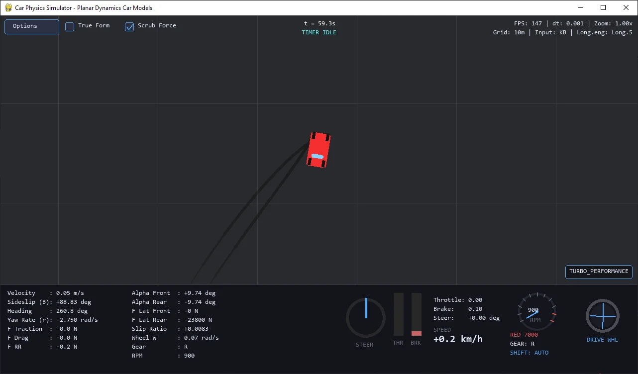
7. Simulator 7 Showcase

Epilogue

If you have made it this far, i suggest you immediately checkout Conclusion of the Macro Monster Car Physics Journey. Things will make a lot more sense for Model 7 and is the canonical conclusion to this series.

Whats more, I’ve decided to reworked the roadmap to basically end at Model 7.5, so, we won’t be having Model 8 for this specific series anymore. To put it bluntly, I think for this series, and the Simulator 7 that I’ve built, Model 7 seems like a good conclusion considering the Macro Monster source this series rely on. But, I don’t plan to outright quit Model 8 just yet, I’m looking to approach it from a different path, with a different reference, stay-tuned for my quick announcement post about that soon.