Car Physics - Model 6: Low-Speed Kinematic Turning
Table of Content
Block
- Main reference: Marco Monster’s Car Physics
- Github repo for Longitudinal Simulators: duy-phamduc68/Longitudinal-Car-Physics
- Github repo for Simulator 6: duy-phamduc68/Planar-Kinematic-Car-Model
- Github repo for Planar Dynamic Simulator(s): duy-phamduc68/Planar-Dynamic-Car-Model
Roadmap
Block
- Model 1: Longitudinal Point Mass (1D)
- Straight Line Physics
- Magic Constants
- Braking
- Model 2: Load Transfer Without Traction Limits (1D)
- Weight Transfer
- Model 3: Engine Torque + Gearing without Slip (1D)
- Engine Force
- Gear Ratios
- Drive Wheel Acceleration (simplified)
- Model 4: Wheel Rotational Dynamics (1D)
- Drive Wheel Acceleration (full)
- Torque on the Drive Wheel & The Chicken and The Egg
- Model 5: Slip Ratio + Traction Curve (1D)
- Slip Ratio & Traction Force
- Model 6: Low-Speed Kinematic Turning (2D)
- Curves (low speed)
- Model 7: High-Speed Lateral Tire Model (2D)
- High Speed Turning
- Model 8: Full Coupled Tire Model (2D)
Model 6 Recap
Model 6 adds 2D kinematic turning: steering now curves the car’s path via geometric constraints, while all the longitudinal physics from Models 1-5 continue to govern speed and traction. It introduces a new state: $\theta$ (heading).
In Model 1, we learned that for a realistic driving experience, we don’t translate throttle -> speed directly. Rather, it’s an interplay between velocity, acceleration, resistance… and most importantly, how fast we can go at any point depends on the scenario rather than only our input. It’s not like we floor the gas and immediately zoom to top speed.
In Model 6, the concept of steering is kinda the same. Now we steer with a generic “left/right” control, but it doesn’t immediately snap our direction to a new angle. Instead, it sets the rate at which we turn, which still depends on velocity and so on. This sets the framework for steering to behave differently at different speeds. For Model 6, we will be looking at this behavior only at low speed, and we accept that this kinematic approximation will break down at high speed until we move to subsequent models on the roadmap.
In Marco Monster’s words, this model is trying to simulate “parking movement”. Parking is usually done at low speed, and the driver usually has very predictable control over the car in this state. The wheels roll where they point, and sideways slip is negligible.
In this post, we are going to implement the framework for our simulator to go from a single 1D line to a 2D plane, and explore a “cheat”, much like in Model 3 and 4, that allows us to isolate heading. In essence, Model 6 (and most models before we reach Model 8) will be built on the philosophy that we separate longitudinal and lateral dynamics.
Even though we just finished building Model 5, which was quite complex and built upon everything before it, you can understand that in Model 6, we have to “restart” the lateral complexity as if we are returning to Model 1 levels, just for steering. We aren’t throwing away our longitudinal progress per se; we’re stacking a simple lateral foundation on top of the complex longitudinal engine we’ve already built. Despite having basically built up longitudinal dynamics at 100%, the lateral side is just getting started.
1. Introduction to Curves
The plot below explicitly visualizes the Instantaneous Center of Rotation (ICR), which is where the lines perpendicular to both wheels intersecting at a single point in the distance. This “pivot point” is what the car is actually rotating around.
In a real car, the two front wheels actually turn at different angles so they don’t scrub (see Ackermann Steering). This “Bicycle Model” simplifies them into one middle wheel as seen in the plot above, try imagining the wheelbase $L$ as the bicycle frame.
Let’s build intuition for what steering actually does geometrically. The interactive plot below shows the core relationship that drives all of Model 6.
1.1. Top Plot: Instantaneous Geometry
This is the car at a single moment in time, viewed from above:
- Blue line (Rear Wheel): The rear axle position. In our bicycle model, this is where the car “pivot point” lives. The rear wheels don’t steer, so they define the car’s reference orientation.
- Orange dotted line (Wheelbase $L$): The distance between front and rear axles. This is a fixed property of the car (~2.5-2.8 m for most sports cars).
- Green line (Front Wheel): The steered front wheel, rotated by angle $\delta$ (delta) relative to the car body.
- Purple arc ($\delta$): The steering angle itself, shown visually.
- Black circle marker ($R$): The instantaneous center of rotation - the point where lines extended from the rear and front wheels intersect. This is the center of the circle the car is currently tracing.
1.2. Bottom Plot: Resulting Path
This shows where the car actually goes if you hold the steering angle constant. Notice it’s a clean circular arc, that’s the kinematic assumption in action. No drift, no understeer, just pure geometry.
Use the sliders to explore:
- Increase steering angle $\delta$: The turn radius $R$ shrinks dramatically. At $\delta = 30$°, you’re doing a tight U-turn. At $\delta = 1 \approx 3$°, you’re barely curving.
- Increase wheelbase $L$: The turn radius grows. This is why long vehicles (trucks, limos) have wider turning circles, this is purely geometry.
1.3. The Key Equation: Steering Angle
The relationship you’re watching in real-time is:
Block
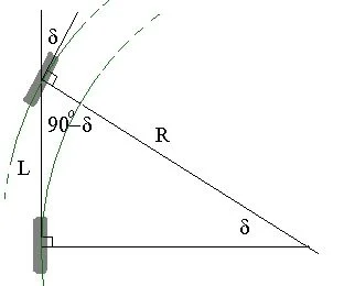
This is pure trigonometry. Look at the top plot: the wheelbase $L$ is the side opposite angle $\delta$ in a right triangle, and $R$ is the hypotenuse. Therefore $sin ( \delta ) = L / R$, which rearranges to the equation above.
Intuition checks:
- If $\delta = 0$° (straight ahead), $sin(0) = 0$, so $R = \infty$ - an infinite radius is a straight line.
- If $\delta \rightarrow 90$° (wheels turned fully sideways), $sin(90°) = 1$, so $R = L$, the car would pivot around the rear axle. (Don’t try this in real life. In the plot above I allow it just for funsies, usually steering angle is limit in the range between $\pm 25 - 45$ degrees.)
- Small $\delta$ -> large $R$ (gentle highway curve). Large $\delta$ -> small $R$ (parking lot turn).
In Model 1-5, the car lived on a 1D line. Position was a scalar, and “turning” didn’t exist. Now we’re on a 2D plane, and steering input doesn’t snap the car to a new direction, it sets the curvature of the path the car will follow.
The turn radius R tells us the shape of the path, but not how fast we’re turning along it. That’s the next piece: converting radius into yaw rate, which then integrates into heading. But before we get there, make sure you’re comfortable with this geometric foundation. The rest of Model 6 is just chaining relationships from this starting point.
2. From Geometry to Motion
In the previous section, we derived the turn radius $R$ from steering angle $\delta$. That tells us the shape of the path, but not how fast we’re traveling along it. To actually move the car, we need to convert that geometric curve into rotational motion, then into world-space position.
2.1. Yaw Rate
If you’re driving at speed $v$ around a circle of radius $R$, how quickly does your heading change? This is the yaw rate $r$ (also called angular velocity, measured in rad/s):
Block
Substituting our turn radius equation $R = L / sin(\delta)$:
Block
This is where velocity matters. At the same steering angle:
- At 10 km/h, you get a slow, lazy rotation
- At 100 km/h, the same steering input produces a yaw rate 10× faster
This is why high-speed turns feel so much more dramatic, and also why our kinematic model will eventually break down at speed (Model 7 will fix this by adding lateral tire forces).
2.2. Heading
In Model 1, we integrated acceleration to get velocity, then integrated velocity to get position:
Block
Now we do the same thing for rotation. Heading $\theta$ is our new state variable, we store it and update it each frame by integrating yaw rate:
Block
Important distinction:
- $\theta$ (heading) is a state: we integrate it over time
- $r$ (yaw rate) is not a state (yet): we compute it fresh each frame from current $v$ and $\delta$
This mirrors Model 4, where we formally introduced wheel rotation $\omega$ as a state but still used the constraint $v = \omega R$ to keep things solvable. Here, we’re using the kinematic constraint $r = v \cdot sin(\delta)/L$ instead of solving for yaw torque from lateral forces. That comes in Model 7.
2.3. World-Space Velocity
In Models 1-5, velocity was a scalar, just speed along a 1D line, now it’s a 2D vector. But here’s the kinematic simplification that defines Model 6:
BlockThe velocity vector always aligns with the car’s heading. No sideslip, no drifting. The car points where it’s going.
This is the “parking lot” assumption Marco Monster mentions. At low speeds, wheels roll where they point. We’ll break this assumption in Model 7.
To move the car in world space, we take the longitudinal speed $v_{long}$ (computed from all our Model 1-5 physics: engine, drag, slip ratio, etc.) and rotate it by the heading angle $\theta$:
Block
This is basic trigonometry: the x-component is $v \cdot cos(\theta)$, the y-component is $v \cdot sin(\theta)$.
2.4. Position Update
Finally, we integrate velocity to get position, just like in Model 1, but now in 2D:
Block
2.5. The Full Chain
Let’s trace the complete flow from user input to car movement:
- Steering input: $\delta$ (steering angle, clamped to $\pm \delta_{max}$)
- Geometry: $R = L / sin(\delta)$ (turn radius)
- Longitudinal Velocity: $v_{long}$ (model 1-5)
- Kinematics: $r = v_{long} / R = v_{long} \cdot sin(\delta) / L$ (yaw rate)
- Integration: $\theta \leftarrow \theta + r \cdot dt$ (heading update)
- Rotation: $v_{world} = \left[ \begin{array}{c} v_{long} \cdot cos (\theta), \ v_{long} \cdot sin (\theta) \end{array} \right]$ (world velocity)
- Integration: $p \leftarrow p + v_{world} \cdot dt $ (where $p = \left[ \begin{array}{c} x, \ y\end{array} \right]$ is position)
Steering doesn’t affect speed (in Model 6), but speed affects how fast you turn.
2.6. Implementation Note: The “Cheat”
Remember how Model 4 used $v = ωR$ as a constraint to avoid solving the full rotational dynamics? We’re doing the same thing here, but for lateral motion:
- Model 4 cheat: Assume no longitudinal slip to compute wheel RPM from car speed
- Model 6 cheat: Assume no lateral slip to compute yaw rate from steering geometry
Both cheats isolate one aspect of the physics while deferring the full complexity to later models.
3. Final Takeaways
Unlike Model 5, which introduced complex new force equations and ODEs, Model 6 is primarily about geometric relationships and coordinate transformations. The longitudinal physics remain exactly as derived in Models 1-5; what’s new is how we integrate heading and convert local velocity into world-space motion.
Because the mathematical relationships are relatively simple (pure trigonometry and kinematics), this reference focuses on the implementation structure rather than re-deriving formulas. The key insight is that Model 6 adds a new state variable (heading $\theta$) and uses it to rotate the velocity vector, while all the force calculations stay in the longitudinal domain.
3.1. The Master ODE System
The vehicle is now modeled as a dynamic longitudinal system (unchanged from Models 1-5) coupled with a kinematic lateral system. The lateral motion is constrained by geometry rather than forces.
- The Translational ODE (Chassis Longitudinal)
Block
- The Rotational ODE (Drive Wheels)
Block
- The Kinematic ODE (Heading)
Block
- The World Space ODEs (Position)
Block
3.2. Core Code Implementation
The update loop now solves the longitudinal physics first (to determine speed $v$), then applies the kinematic constraint (to determine yaw rate $r$), and finally integrates position in 2D. To keep the focus on the new turning logic, we collapse Models 1-5 into a single function call.
def update(self, dt, throttle, brake, steering):

    # 1. State from previous frame
    v_prev = self.v
    w_prev = self.omega
    theta_prev = self.theta
    x_prev, y_prev = self.x, self.y

    # 2. Longitudinal Physics (Models 1-5) - COLLAPSED FOR CLARITY
    # This function contains all the Model 5 logic:
    # - Weight transfer calculation
    # - Engine torque lookup and gearing
    # - Slip ratio and traction force
    # - Drag and rolling resistance
    # - Net force and acceleration integration
    # Returns updated longitudinal speed v and wheel speed omega
    self.v, self.omega = self.calculate_longitudinal_physics(
        dt, throttle, brake, v_prev, w_prev
    )

    # 3. Kinematic Turning (Model 6) - THE NEW STUFF

    # Clamp steering angle to physical limits
    delta = clamp(steering * self.DELTA_MAX, -self.DELTA_MAX, self.DELTA_MAX)

    # Calculate yaw rate from geometry: r = v * sin(delta) / L
    # This is the kinematic constraint - no lateral forces involved yet
    yaw_rate = (self.v * math.sin(delta)) / self.L

    # Integrate heading: theta <- theta + r * dt
    # Heading is our new state variable
    self.theta = theta_prev + yaw_rate * dt

    # Rotate velocity from local car space to world space
    # This is where 1D becomes 2D: v_world = R(theta) * [v, 0]^T
    vx_world = self.v * math.cos(self.theta)
    vy_world = self.v * math.sin(self.theta)

    # Integrate position in 2D
    self.x = x_prev + vx_world * dt
    self.y = y_prev + vy_world * dt

    # Return telemetry for the UI
    return {
        'speed': self.v,
        'heading': self.theta,
        'pos': (self.x, self.y),
        'yaw_rate': yaw_rate,
        'slip_ratio': self.slip_ratio
    }


def calculate_longitudinal_physics(self, dt, throttle, brake, v_prev, w_prev):
    """
    This function encapsulates ALL of Models 1-5.
    It takes the previous longitudinal states and returns updated values.
    The implementation is identical to Model 5's update loop.
    """
    # [Insert complete Model 5 logic here]
    # - Calculate dynamic weight transfer
    # - Look up engine torque from RPM curve
    # - Apply gear ratios and transmission efficiency
    # - Calculate slip ratio sigma = (omega*R - v) / max(|v|, epsilon)
    # - Calculate traction force F_t = clamp(C_t * sigma, -F_max, F_max)
    # - Calculate drag F_drag = C_drag * v * |v|
    # - Calculate rolling resistance F_rr = C_rr * v
    # - Calculate net force and acceleration
    # - Integrate v and omega
    # - Return updated v and omega

    # For brevity, showing the final integration step:
    a = self.F_net / self.M
    alpha = self.T_net / self.I_W

    v_new = v_prev + a * dt
    w_new = w_prev + alpha * dt

    return v_new, w_new
4. Simulator 6 - Showcase
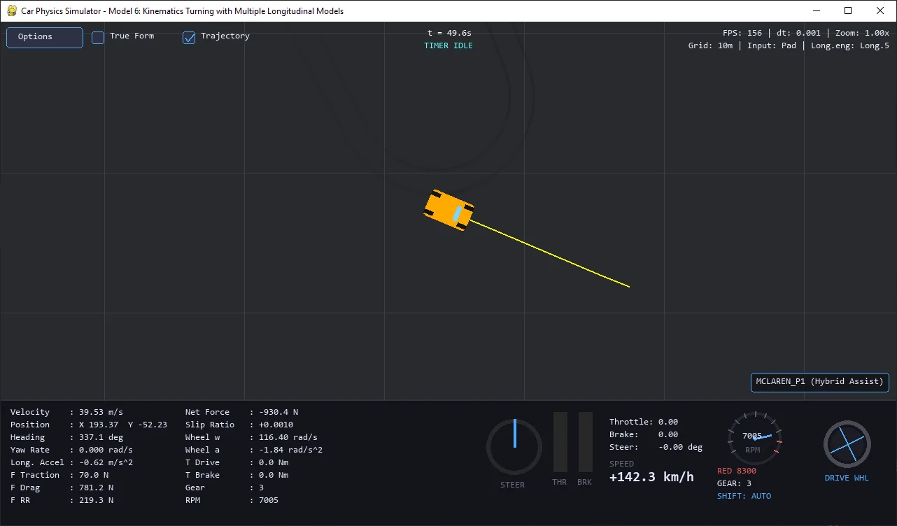
While working on Simulator 6, I noticed it was getting quite complex, so I decided to give it a dedicated repo:
- Github repo for Simulator 6: duy-phamduc68/Planar-Kinematic-Car-Model
Model 7 and 8 will also have their own repo, but I’m really considering to bundle them to a single repo (a single model) for closure, because looking ahead a bit, model 8 just seem more like a clean-up / conclude everything model, so it might be a good idea to just make both into a single model, though I will still have 2 dedicated post for each.