Table of Content

• Table of Content
• Roadmap
• Model 5 Recap
• Slip Ratio
• The Traction Curve
• Phase 1: The “Bite” (Linear Phase)
• Phase 2: The Limit (Saturation Phase)
• Solving the Chicken and Egg
• Final Takeaways
• The Master ODE System
• The Complete Formula Book
• A. Engine & Drivetrain
• B. Slip & Traction
• C. Weight Transfer & Grip Limits
• D. Environmental Resistances & Brakes
• Code Code Implementation
• Simulator 5 - Showcase
• Hybrid Traction Solver
• Virtual Clutch and Stall Dynamics
• Effective Drivetrain Inertia ($I_{eff}$)
• Telemetry Enhancements and UI Improvements

Block

• Main reference: Marco Monster’s Car Physics
• Github repo for Longitudinal Simulators: duy-phamduc68/Longitudinal-Car-Physics
• Github repo for Planar Simulators: duy-phamduc68/Planar-Car-Physics

Roadmap

• Model 1: Longitudinal Point Mass (1D)
  • Straight Line Physics
  • Magic Constants
  • Braking
• Model 2: Load Transfer Without Traction Limits (1D)
  • Weight Transfer
• Model 3: Engine Torque + Gearing without Slip (1D)
  • Engine Force
  • Gear Ratios
  • Drive Wheel Acceleration (simplified)
• Model 4: Wheel Rotational Dynamics (1D)
  • Drive Wheel Acceleration (full)
  • Torque on the Drive Wheel & The Chicken and The Egg
• Model 5: Slip Ratio + Traction Curve (1D)
  • Slip Ratio & Traction Force
• Model 6: Low-Speed Kinematic Turning (2D)
  • Curves (low speed)
• Model 7: High-Speed Lateral Tire Model (2D)
  • High Speed Turning
• Model 8: Full Coupled Tire Model (2D)

Block

Model 5 Recap

Okay so I highly suggest you read through the Model 4: Wheel Rotational Dynamics (1D) post if you haven’t already, especially starting from Slip Ratio Introduction onwards. Specifically, zoom in on:

“And that Slip, actually belongs to model 5.”

“This is kind of a “gotcha” with my roadmap, you technically can’t exactly implement model 4 in isolation like the last 3 models, let’s walk through what would happen if we actually try…”

Block

And we did try in that post, yeah, just anchor on that, and I will continue as if we are simply resuming said paragraph in the model 4’s notes.

In short: we define slip ratio, remove the hack from model 4 (and model 3), and thats about it. This will be a pretty short post in the series.

Let’s do this, we are so close to finishing our longitudinal simulator (1D), and we will move to 2D right after model 5!

Slip Ratio

Since the wheel’s speed ($\omega$) and the car’s speed ($v$) are now fully independent states, we need a mathematical way to measure their disagreement. This is the formal Slip Ratio ($\sigma$):

$$\sigma = \frac{\omega R_w - v}{| v |}$$

Block

Why the absolute value $| v |$? Dividing by the magnitude of the velocity ensures that the sign of the slip ratio remains physically correct even when the car is traveling in reverse.

• The Low-Speed Singularity:

If the car is at a complete standstill ($v = 0$), this equation divides by zero and explodes. In our code, we will have to introduce a small safety clamp, for example, replacing $|v|$ with:

max(abs(v), 0.1)

to prevent the physics engine from crashing when accelerating from a stop.

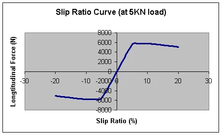
Here, longitudinal force is the same as $F_{traction}$. In Macro Monster’s words:

“Note how the force is zero if the wheel rolls, i.e. slip ratio = 0, and the force is at a peak for a slip ratio of approximately 6 % where the longtitudinal force slightly exceeds the wheel load. The exact curve shape may vary per tyre, per road surface, per temperature, etc. etc.”

“That means a wheel grips best with a little bit of slip. Beyond that optimum, the grip decreases. That’s why a wheel spin, impressive as it may seem, doesn’t actually give you the best possible acceleration. There is so much slip that the longtitudinal force is below its peak value. Decreasing the slip would give you more traction and better acceleration.”

Block

The Traction Curve

Now that we have a percentage of “stretch” ($\sigma$), we must convert it into actual Newtons of pushing force ($F_{traction}$).

Real tires have highly complex, non-linear curves (like the Pacejka Magic Formula). For Model 5, we use a robust Linear Approximation with a Cap:

Phase 1: The “Bite” (Linear Phase)

For small amounts of slip, the tire acts like a stiff rubber band. The relationship is proportional:

$$F_{traction} = C_t \cdot \sigma$$

Block

• $C_t$ is the Traction Stiffness. This is typically a massive number (e.g., 100,000 N per 1.0 slip), meaning even a tiny 5% slip generates a massive amount of forward force.

Phase 2: The Limit (Saturation Phase)

A tire is not magic; eventually, the rubber gives up and slides. The absolute maximum grip the tire can provide is dictated entirely by the weight pressing down on it. This is where Model 2 (Load Transfer) finally proves its worth!

$$F_{max} = \mu \cdot W_{driveAxle}$$

Block

• $\mu$ is the coefficient of friction (e.g., 1.0 for dry asphalt).
• $W_{driveAxle}$ is the dynamic load on the drive wheels (e.g., $W_r$ for a rear-wheel-drive car), which shifts backward when you accelerate!

To get our final force, we simply calculate the linear “bite” and clamp it to the physical limits of the tire:

$$F_{traction} = \text{Clamp}(C_t \cdot \sigma, -F_{max}, F_{max})$$

Block

Solving the Chicken and Egg

We no longer need the Model 4’s hack. The engine never talks directly to the road anymore. We solve the “Chicken and Egg” problem by using the previous frame’s values to calculate the current frame’s forces.

Here is the new, fully decoupled execution order:

1. Calculate Slip: Compare current $\omega$ and $v$ to find $\sigma$.
2. Calculate Traction: Convert $\sigma$ to $F_{traction}$, capped by $F_{max}$.
3. Push the Chassis: Apply $F_{traction}$ to the Translational ODE to accelerate the car body ($v$).
4. Resist the Wheels: Convert $F_{traction}$ into a resistive torque ($T_{traction} = F_{traction} \cdot R_w$) and apply it to the Rotational ODE to fight the engine’s $T_{drive}$.

Final Takeaways

This section serves as the definitive reference for the completed Longitudinal Vehicle Dynamics System (Models 1–5). It documents the final decoupled Ordinary Differential Equations (ODEs), the complete formula book, and the step-by-step algorithmic loop required to simulate a car in one dimension.

The Master ODE System

The vehicle is modeled as two separate physical entities, the chassis and the drive wheels, that interact exclusively through the tire contact patch.

• The Translational ODE (Chassis)

$$\frac{dv}{dt} = \frac{1}{M} \left( F_{traction} - F_{drag} - F_{rr} \right)$$

Block

• The Rotational ODE (Drive Wheels)

$$\frac{d\omega}{dt} = \frac{1}{I_w} \left( T_{drive} - T_{brake} - T_{traction} \right)$$

Block

The Complete Formula Book

To solve the master ODEs, we must calculate the specific forces and torques at every timestep.

A. Engine & Drivetrain

The engine generates torque based on the current wheel speed, gear ratios ($x_g$, $x_d$), and throttle input ($u$).

$$rpm = \max \left( \omega \cdot x_g \cdot x_d \cdot \frac{60}{2\pi}, RPM_{idle} \right)$$

Block

$$T_{drive} = u \cdot T_{engine}(rpm) \cdot x_g \cdot x_d \cdot \eta$$

Block

B. Slip & Traction

The difference between the wheel’s surface speed and the car’s true speed creates rubber deformation, yielding force.

$$\sigma = \frac{\omega R_w - v}{\max(|v|, \epsilon)}$$

Block

(Where $\epsilon$ is a small value like $0.1$ to prevent division by zero at a standstill)

$$F_{traction} = \text{clamp}(C_t \cdot \sigma, -F_{max}, F_{max})$$

Block

$$T_{traction} = F_{traction} \cdot R_w$$

Block

C. Weight Transfer & Grip Limits

The maximum possible traction ($F_{max}$) is capped by the dynamic weight pushing down on the drive axle (assuming RWD).

$$W_r = \left( \frac{b}{L} M g \right) + \left( \frac{h}{L} M a_{prev} \right)$$

Block

$$F_{max} = \mu \cdot W_r$$

Block

D. Environmental Resistances & Brakes

Forces that perpetually oppose the motion of the chassis and the rotation of the wheels.

$$F_{drag} = C_{drag} \cdot v \cdot |v|$$

Block

$$F_{rr} = C_{rr} \cdot v$$

Block

$$T_{brake} = \text{sgn}(\omega) \cdot B \cdot C_{brakeTorque}$$

Block

Code Code Implementation

Because $F_{traction}$ depends on $v$ and $\omega$, and $v$ and $\omega$ depend on $F_{traction}$, we solve the system numerically. We use the states from the start of the frame to calculate all forces, and then integrate to find the states for the next frame.

def update(self, dt, throttle, brake):
    
    # 1. State from previous frame
    v_prev = self.v
    w_prev = self.omega
    a_prev = self.a  # Needed for dynamic load transfer
    
    # 2. Dynamic Grip Limit (Model 2)
    W_r = (self.b / self.L) * self.M * self.g + (self.h / self.L) * self.M * a_prev
    F_max = self.MU * W_r
    
    # 3. Engine & Drivetrain Torque (Model 3)
    rpm = max(w_prev * self.gear_ratio * self.final_drive * (60 / (2 * math.pi)), self.RPM_IDLE)
    T_engine = throttle * get_max_torque(rpm)
    T_drive = T_engine * self.gear_ratio * self.final_drive * self.ETA
    
    # 4. Slip & Traction Force (Model 5)
    # Use max(abs(v_prev), 0.1) to avoid divide-by-zero when completely stopped
    slip_ratio = (w_prev * self.R_W - v_prev) / max(abs(v_prev), 0.1)
    
    F_traction_raw = self.C_t * slip_ratio
    F_traction = clamp(F_traction_raw, -F_max, F_max)
    T_traction = F_traction * self.R_W
    
    # 5. Resistances & Braking
    F_drag = self.C_DRAG * v_prev * abs(v_prev)
    F_rr = self.C_RR * v_prev
    
    T_brake = 0.0
    if abs(w_prev) > 0.01:
        T_brake = brake * self.C_BRAKE_TORQUE * math.copysign(1.0, w_prev)
    
    # 6. Solve Master ODEs (Model 4/5 integration)
    F_net = F_traction - F_drag - F_rr
    T_net = T_drive - T_brake - T_traction
    
    self.a = F_net / self.M
    alpha = T_net / self.I_W
    
    # 7. Integrate States
    self.v = v_prev + self.a * dt
    self.omega = w_prev + alpha * dt
    self.x = self.x + self.v * dt
    
    # Return telemetry for the UI
    return self.a, F_traction, slip_ratio, self.omega, T_drive, T_traction

Simulator 5 - Showcase

Simulator 5 represents the culmination of our 1D physics exploration, combining academic Ordinary Differential Equations (ODEs) with a practical, stable video game physics engine. By removing the “Effective Mass Hack” from Model 4, the chassis and drive wheels now function as independent entities, dynamically interacting through a responsive contact patch.

Raw ODEs at low speeds can lead to issues like division by zero and jitter. Simulator 5 mitigates these problems with safeguards, smoothing algorithms, and mechanical adjustments.

Hybrid Traction Solver

To address vibrations at $0$ m/s caused by hypersensitive slip ratios, we implemented a dual-state traction system:

• Sticky Mode: When external torque is below the tire’s physical limit ($F_{max}$), the simulator bypasses the slip formula, locking the wheels to the road for smooth creeping and precise braking.
• Slip Mode: When torque exceeds the tire’s grip, the engine transitions to the Model 5 ODEs, allowing the wheels to spin out or lock up independently of the chassis.

Virtual Clutch and Stall Dynamics

Simulator 5 introduces a virtual clutch to replace Model 4’s engine that never dropped below idle:

• Launching (1st Gear): The clutch slips intentionally, allowing the engine to rev up and transfer torque smoothly, enabling burnouts.
• Stalling (5th Gear): Attempting to launch in a high gear results in the tires overpowering the engine, dragging RPM to $0$ and stalling the car.

Effective Drivetrain Inertia ($I_{eff}$)

To prevent RPM oscillations when traction breaks, the engine’s internal mass is scaled through the transmission gearing:

$$I_{eff} = I_w + I_{engine} \cdot (\text{Gear Ratio} \cdot \text{Final Drive})^2$$

Block

This adjustment makes the wheels feel “heavier” in lower gears, acting as a shock absorber for RPM jitter and simulating shift-lock skidding during abrupt downshifts.

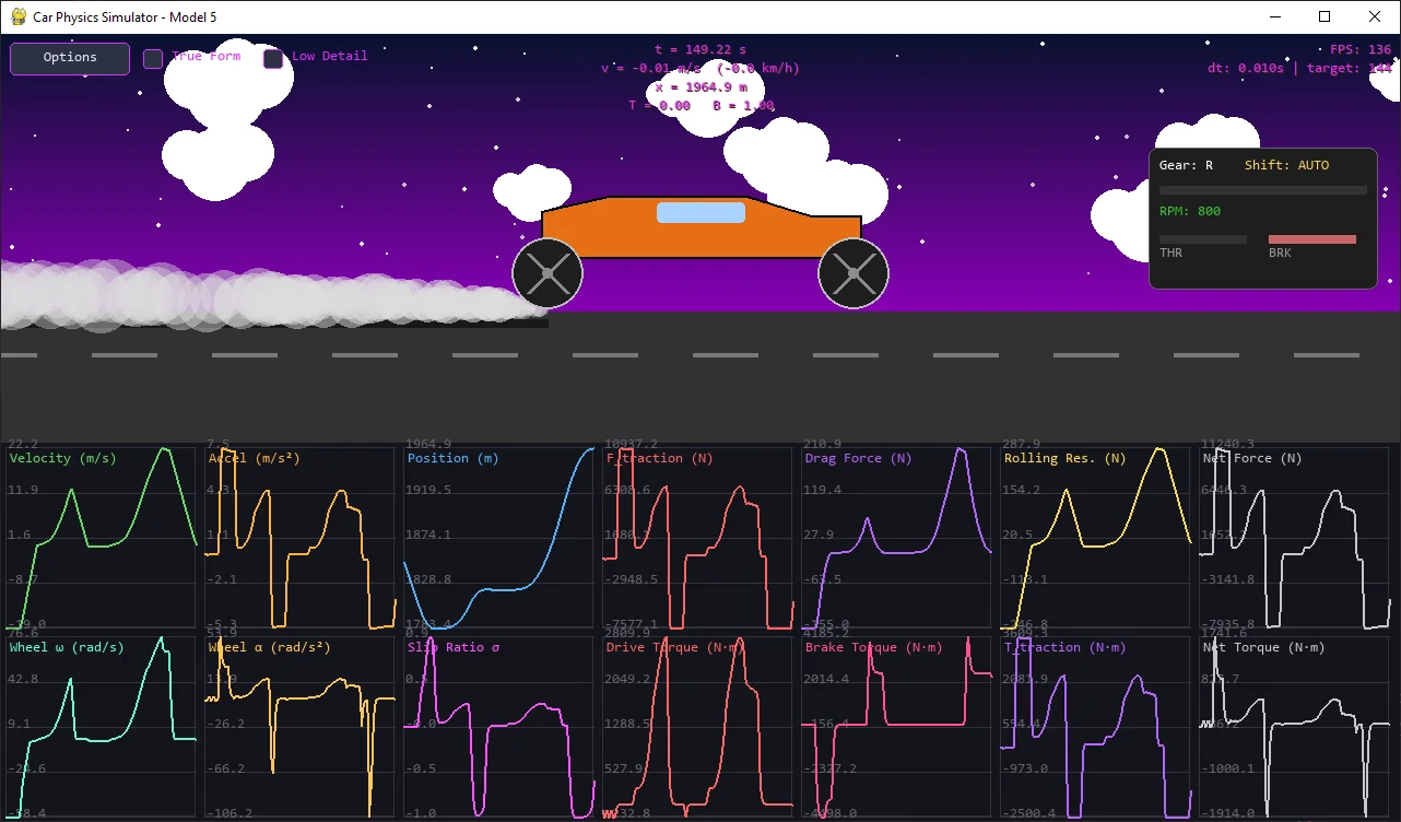
Telemetry Enhancements and UI Improvements

Raw physics data is noisy, so we refined the telemetry and visuals for a clearer driver experience:

• EMA Filtered Graphs: The GraphBuffer applies an Exponential Moving Average (EMA) algorithm, smoothing chaotic raw data into clean, readable graphs while preserving pixel-perfect accuracy for position and velocity.
• Dual RPM Gauge: The dashboard now features two RPM bars: a thick green bar for Engine RPM and a thin cyan bar for Wheel RPM, making clutch slips and brake lock-ups instantly visible.
• Dynamic Visuals: Optimized skid marks, alpha-blended tire smoke, and a flashing “SLIP” warning enhance the HUD whenever the tires exceed $F_{max}$.

Check out the simulator at duy-phamduc68/Longitudinal-Car-Physics.

I ain’t gonna lie, I don’t really know what to say here, I just know that we are moving to 2D / Planar physics soon, which means longitudinal + lateral dynamics :). Right now, I’m a bit tired. I will be studying it and complete this thing real soon, see you then.