Table of Content

• Table of Content
• Roadmap
• Model 4 Recap
• Looking back at previous models
• System Graph: Model 2
• System Graph: Model 3
• System Graph: Model 4
• Throwback: States
• Wheel Speed Calculation
• Torque Calculation
• A System of Ordinary Differential Equations
• How to Calculate Torque
• Coupling and Relation to Model 5
• Traction Force
• Slip Ratio Introduction
• The Need for Model 5
• Simulator 4
• Actual Changes
• Simulator 4 - Showcase
• Final Takeaways
• The Updated Implementation
• Towards Model 5

Block

• Main reference: Marco Monster’s Car Physics
• Main Github repo: duy-phamduc68/Car-Physics

Roadmap

• Model 1: Longitudinal Point Mass (1D)
  • Straight Line Physics
  • Magic Constants
  • Braking
• Model 2: Load Transfer Without Traction Limits (1D)
  • Weight Transfer
• Model 3: Engine Torque + Gearing without Slip (1D)
  • Engine Force
  • Gear Ratios
  • Drive Wheel Acceleration (simplified)
• Model 4: Wheel Rotational Dynamics (1D)
  • Drive Wheel Acceleration (full)
  • Torque on the Drive Wheel & The Chicken and The Egg
• Model 5: Slip Ratio + Traction Curve (1D)
  • Slip Ratio & Traction Force
• Model 6: Low-Speed Kinematic Turning (2D)
  • Curves (low speed)
• Model 7: High-Speed Lateral Tire Model (2D)
  • High Speed Turning
• Model 8: Full Coupled Tire Model (2D)

Block

Model 4 Recap

In model 3, we assumed that:

$$v = \omega_{wheel} \cdot R_w$$

Block

And in model 4, we remove that constraint, and we make $ \omega_{wheel} $ an actual state, sort of “separate” it from the car, meaning that, wheel speed and car speed can differ, intuitively, you can think about cases like:

• The car is zooming and tires lose traction
• Going at high speed then hit the brakes, the tires won’t just slow down immediately.

Think of model 4 as like a “setup” for such cases because actually such behavior will emerge when we get to model 5.

Looking back at previous models

System Graph: Model 2

From this, we see that:

• Force is “injected magically”
• A simple “thrust” power to move the car.
• Load transfer is currently disconnected from motion.

Basically, F_engine just spawns out of thin air.

System Graph: Model 3

For model 3, engine is now causal and realistic, but the wheels are still fake (check post on model 3 about the glued wheels), and the drivetrain is basically a function like:

F_drive = f(v, gear, throttle)

And different from model 2, model 3 doesn’t necessarily spawn anything from thin air, but:

$$v = \omega_{wheel} \cdot R_w$$

Block

is a convenient constraint, not physics.

System Graph: Model 4

The crucial detail here is that model 3 collapse everything into one loop:

v -> rpm -> torque -> force -> a -> v

While in model 4, we have:

Path A (translational):
torque -> force -> acceleration -> v

Path B (rotational):
torque -> angular accel -> ω -> rpm -> torque

And these two are only loosely coupled together (might give you some hint about future models! specifically loosely coupled vs fully coupled).

Throwback: States

To truly understand the core of model 4, we have to go way back to model 1, and in a way, undermine model 2 and 3.

You might have forgotten about states, thats understandable, because in model 2 and 3, we didnt really introduce any new states nor mention them. In Model 1: Longitudinal Point Mass (1D), we defined:

• $x(t) \geq 0$ : Position of the car. Meters (m).
• $v(t) = \frac{dx}{dt}$ : Velocity or the car. Meters per second (m/s).
• $a(t) = \frac{dv}{dt}$ : Acceleration of the car. Meters per second squared (m/s²).

Note that $a(t)$ is more like a derivation than a state here, its the rate of change of $v$, so derived from $v(t)$, therefore, since model 1, we defined our model with 2 states. In model 4, we introduce another state: $\omega$ (wheel speed / rotational speed), so now, our states consist of:

• $x(t) \geq 0$ : Position of the car. Meters (m).
• $v(t) = \frac{dx}{dt}$ : Velocity or the car. Meters per second (m/s).
• $\omega (t)$ : Angular velocity of the drive wheels. Radians per second (rad/s).

Now, just as how $a$ is derived from $v$, we have another type of acceleration $\alpha$ that is derived from our new state $\omega$:

• $a(t) = \frac{dv}{dt}$ : Linear Acceleration of the car. Meters per second squared (m/s²).
• $\alpha(t) = \frac{d\omega}{dt}$ : Angular Acceleration of the car. Radians per second squared (rad/s²).

So as you can see, if in model 3, we have the constraint:

$$v = \omega_{wheel} \cdot R_w$$

Block

which imply that the wheels are the car are essentially “the same”, then now in model 4, we explicitly state that the car and the wheels are formally and physically separate - as it should.

Wheel Speed Calculation

Now that we have sever the shortcut in model 3, to get $\omega$, you are gonna use a very familiar formula again:

$$\alpha = \frac{T}{I} \quad (1)$$

Block

This is actually the rotational equivalent for Newton’s Second Law, where:

• $ \alpha $ : Angular acceleration (rad/^s)
• $ T $ : Torque (N.m)
• $ I $ : Moment of Inertia (kg.m²)

Now you can really see how we are going through a very similar process as in Model 1: Longitudinal Point Mass (1D):

Let’s rewrite $(1)$ to be more fitting for our notation:

$$\alpha = \frac{T_{net}}{I_w}$$

Block

Thus giving us a new ODE:

$$T_{net} = I_w \cdot \alpha (t) = I_w \cdot \frac{d \omega}{dt} \\ \frac{d \omega}{dt} = \frac{1}{I_w} (T_{drive} + T_{brake} + T_{traction})$$

Block

And just like how we used Euler’s method to get velocity, we do the same to get wheel speed:

• Step 1: Start with the angular derivative definition

$$\frac{d\omega}{dt} \approx \frac{\omega_{new} - \omega_{old}}{\Delta t}$$

Block

• Step 2: Substitute the Rotational ODE

$$\frac{\omega_{new} - \omega_{old}}{\Delta t} = \frac{T_{net}(\omega_{old}, v_{old})}{I_w}$$

Block

Note: $T_{net}$ depends on both wheel speed and vehicle velocity, this is called coupling, we will address that in the next section.

• Step 3: Solve for $\omega_{new}$

$$\omega_{new} = \omega_{old} + \Delta t \cdot \frac{T_{net}(\omega_{old}, v_{old})}{I_w}$$

Block

Torque Calculation

A System of Ordinary Differential Equations

So now we have the rotational and translational equations:

$$\frac{d \omega}{dt} = \frac{1}{I_w} \left(T_{drive} + T_{brake} + T_{traction} \right) \\[10pt] \frac{dv}{dt} = \frac{1}{m} \left(F_{traction} + F_{resist} + F_{braking} \right)$$

Block

That second equation, the one governing $v$, that was our master ODE from model 1 up until model 3, but now, it will have to change:

$$\frac{d \omega}{dt} = \frac{1}{I_w} \left(T_{drive} + T_{brake} + T_{traction} \right) \\[10pt] \frac{dv}{dt} = \frac{1}{m} \left(F_{traction} + F_{resist} \right)$$

Block

Throughout model 1 - model 3, we had a magical $F_{braking}$ that somehow just “stops/slows down” the car, but in reality, the brakes act on the wheels, therefore, $F_{braking}$ is completely removed from the second equation, and lives as $T_{brake}$ in the first one instead.

This is whats called a Coupled System of First-Order Ordinary Differential Equations. I won’t really go in depth into the differential equations stuff here, not in this post at least, when I’m finished with model 8, I might come back to derive everything empirically again, maybe.

For now, just think about these 2 equations as how we are explicitly modelling the car and the wheels separately. I’ll call them the Translational ODE (T-ODE) and Rotational ODE (R-ODE). They also establish the car physically: force (linear) mean the road, the air and the car acting on eachother, torque mean the engine and the wheels acting on eachother (and the gears).

How to Calculate Torque

The rotational ODE governs $\omega_{wheel}$, we calculate $ T_{net}$ to find angular acceleration:

$$T_{drive} = u \cdot T_{engine}(rpm) \cdot x_g \cdot x_d \cdot n$$

Block

Resistance of the road exerts back onto the spinning wheels:

$$T_{traction} = -F_{traction} \cdot R_w \quad (2)$$

Block

The fact that $F_{traction}$ shows up in this formula is why this system is coupled, the R-ODE depends on a variable from the T-ODE, we will explore that coupling in the next section.

and resistive torque from the brakes:

$$T_{brake} = - sgn(\omega) \cdot B \cdot C_{brakeTorque}$$

Block

remember that our brake is analog since model 3. $C_{brakeTorque}$ is the maximum clamping force of the brake, measured in N.m

Coupling and Relation to Model 5

Traction Force

Take a look at this diagram:

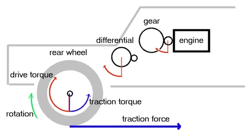
This explains $(2)$ a lot, for example, traction torque will always oppose drive torque, but most importantly, is that we can only know traction torque if we know traction force.

In the T-ODE, our $F_{resist}$ formula remains the same:

$$F_{resist} = F_{drag} + F_{rr} = - C_{drag} \cdot v \cdot |v| - C_{rr} \cdot v$$

Block

However, you might have noticed that before, we used $F_{drive}$ to explain motion, more specifically in model 3, we had:

$$F_{drive} = \frac{u \cdot T_{engineMax} \cdot x_g \cdot x_d \cdot n}{R_w}$$

Block

Now, we don’t have that anymore, it lives in $T_{drive}$ as torque now, as it should. What we have replaced it with is $F_{traction}$, which is the force representing (in forward motion):

• the wheel pushing backward on the road surface
• in reaction, the road pushes forward on the wheel
• this physically moves the car mass ($m$)

Therefore, as seen in the MM diagram, $F_{traction}$ moves the car forward, while $T_{traction}$ is actually a resistance here. This is when we establish $F_{traction}$ as the bridge between the two ODEs.

Slip Ratio Introduction

If $F_{traction}$ isn’t just calculated from the engine torque, how do we know how much force the road is giving us?

The road only pushes back if it feels the tire “scraping” or “stretching” against it. This is the concept of Slip.

Imagine the car is moving at $10~m/s$ ($v$), but the engine is spinning the wheels at a surface speed of $11~m/s$ ($\omega \cdot R_w$). That $1~m/s$ difference means the rubber is literally scraping against the asphalt.

• No Slip ($\omega R_w = v$): This was model 3, the tire is just rolling perfectly. The road doesn’t feel a “push,” so $F_{traction}$ is zero.
• Positive Slip ($\omega R_w > v$): The wheels are spinning faster than the car. This generates forward $F_{traction}$ to accelerate the car.
• Negative Slip ($\omega R_w < v$): The wheels are spinning slower (braking). This generates backward $F_{traction}$ to slow the car down.

This “scraping” or “difference in speeds” is standardized as the Slip Ratio ($\sigma$).

The Need for Model 5

In Model 4, we establish the Rotational ODE to track the wheel speed ($\omega$) as an independent state. However, this creates a “Chicken and Egg” problem:

• To calculate the wheel’s acceleration ($\alpha$), we need Traction Torque ($T_{traction}$).
• Traction Torque comes from Traction Force ($F_{traction}$).
• In a real car, $F_{traction}$ is determined by Slip

And that Slip, actually belongs to model 5.

This is kind of a “gotcha” with my roadmap, you technically can’t exactly implement model 4 in isolation like the last 3 models, let’s walk through what would happen if we actually try, lets say if we leave out the current bottleneck, $F_{traction}$, meaning that $F_{traction} = 0$ at all times, then:

$$\frac{d \omega}{dt} = \frac{1}{I_w} \left(T_{drive} + T_{brake} + 0 \right) \\[10pt] \frac{dv}{dt} = \frac{1}{m} \left(0 + F_{resist} \right)$$

Block

Now what does this mean? Even though we can still input $u$ and $B$, and they will produce a non-zero net torque, it actually only affects the wheel speed $\omega_{wheel}$, literally nothing is updating $v$, the actual car speed. So, its kinda like that contraption from Pixar’s Cars 3:

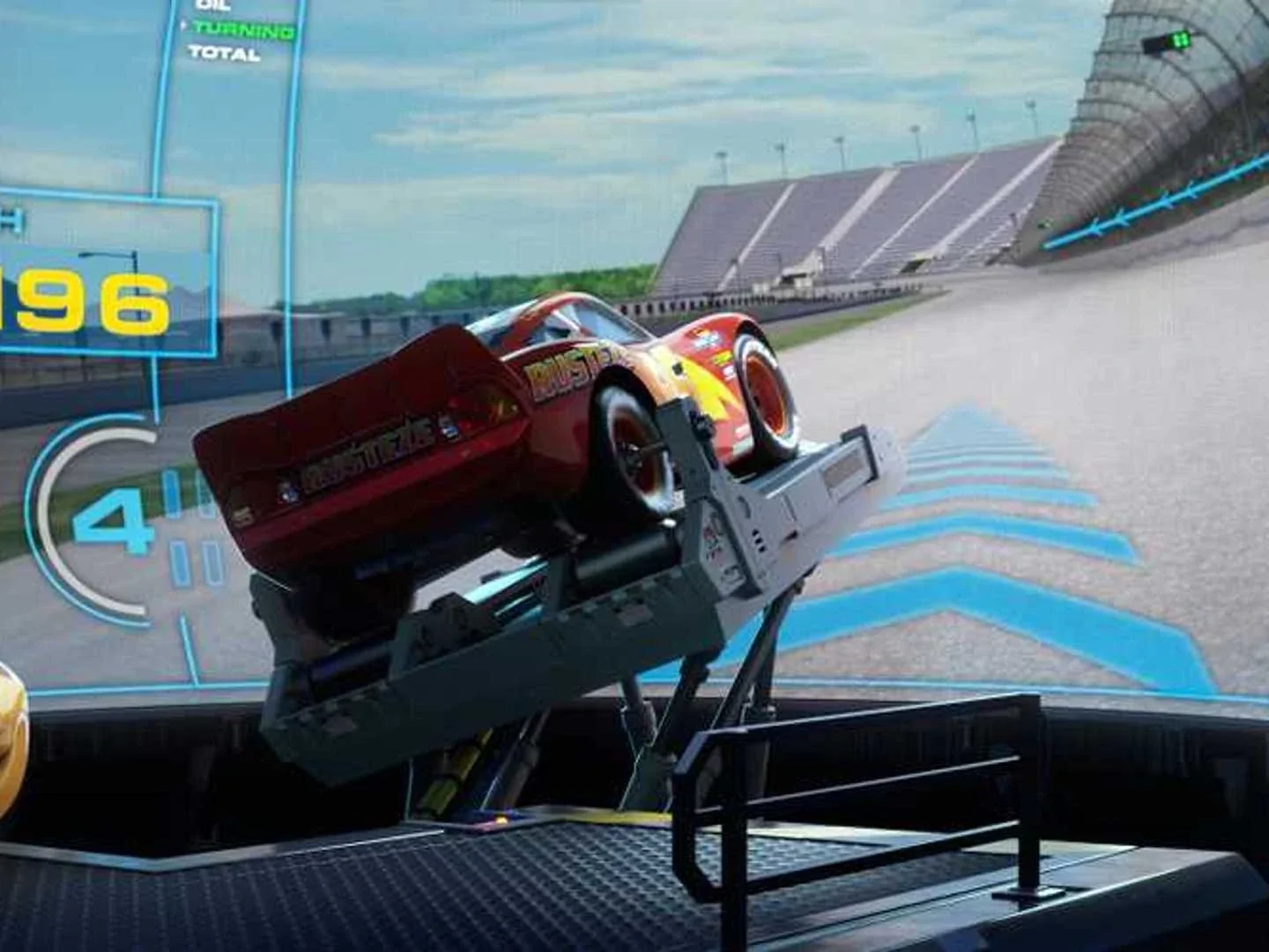
Your wheels will be spinning incredibly fast very quickly, but you won’t go anywhere, you literally cannot move from a standstill, ie. $v$ = 0. (your wheels will spin very quickly if you hit the gas because you are only fighting the inertia $I_w$, usually only about 0.5 - 2.0 kg.m², the car’s mass $m$ is irrelevant in this case).

Bonus: if the car somehow was already moving, ie $v \neq 0 $, then that $F_{resist}$ term will make it stop very quickly and you won’t be able to move again.

Simulator 4

Actual Changes

So, we actually still need the constraint from model 3:

$$\omega_{wheel} = \frac{v}{R_w}$$

Block

which will give us:

$$\alpha = \frac{a}{R_w}$$

Block

This is kind of a cheat, while I did say from the very start of the post that we will remove this constraint, and technically we did when we introduced the new system of ODE with T-ODE and R-ODE, and we will make it complete model 5. For model 4 simulator to actually function, we still need to implement that constraint.

The good news is, model 4’s simulator will be different from simulator 3, just… by a hair.

In model 3, we calculated $a$ with:

$$a = \frac{1}{m} \cdot \frac{f\left(\frac{v}{R_w} \cdot x_g \cdot x_d \cdot \frac{60}{2 \pi} \right) \cdot x_g \cdot x_d \cdot n}{R_w}$$

Block

in model 4, it will become:

$$a = \frac{\frac{T_{drive}}{R_w} + F_{drag} + F_{rr}}{M + \frac{I_w}{R_w^2}}$$

Block

Still, even though it seems underwhelming, our state vector still formally include 3 components now:

• $x(t)$
• $v(t)$
• $\omega (t)$

Simulator 4 - Showcase

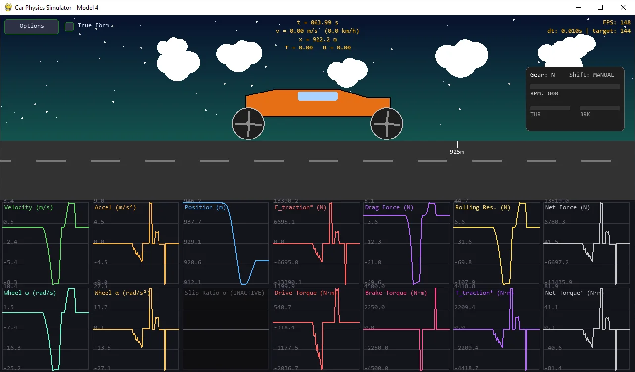
The variables that were “cheated” has an asterisk next to them.

Final Takeaways

This section wraps up Model 4: Wheel Rotational Dynamics by summarizing the transition from kinematics to true rotational dynamics, the temporary constraint we used, and what limitations remain.

Model 4 fundamentally changes the system by separating the car body and the wheels into two distinct physical entities that communicate through the contact patch.

1. The Rotational ODE (The Wheel)

$$\frac{d\omega}{dt} = \frac{1}{I_w} \left( T_{drive} - T_{traction} - T_{brake} \right)$$

Block

2. The Translational ODE (The Chassis)

$$\frac{dv}{dt} = \frac{1}{M} \left( F_{traction} - F_{drag} - F_{rr} \right)$$

Block

Crucial Changes:

• $F_{braking}$ is gone from the linear equation. Brakes now apply Torque ($T_{brake}$) to the wheels.
• The engine outputs Torque ($T_{drive}$), not linear force.
• $F_{traction}$ is the single mathematical “bridge” connecting the two equations ($T_{traction} = F_{traction} \cdot R_w$).

Because we do not yet have a formula for $F_{traction}$ (which requires Model 5’s slip mechanics), solving the two ODEs independently would result in the wheels spinning infinitely in a vacuum.

To make the car drivable, Model 4 temporarily retains the “Suction Cup” constraint ($v = \omega R_w$), algebraically merging the two ODEs into one:

$$a = \frac{ \frac{T_{drive} - T_{brake}}{R_w} - F_{drag} - F_{rr} }{ M + \frac{I_w}{R_w^2} }$$

Block

By using this hack, the engine torque is converted directly to force, but it must now push the Effective Mass of the system: the car’s mass ($M$) plus the “virtual weight” of the spinning wheels ($\frac{I_w}{R_w^2}$).

The Updated Implementation

The physics loop now calculates torque, integrates using the effective mass, and elegantly back-calculates the static friction (Traction Torque) to keep the UI perfectly physically accurate.

# === CONSTANTS (from Model 4) ===
M = 1500            # kg
I_W = 3.0           # kg·m^2 (Rotational inertia of drive wheels)
R_W = 0.33          # m
C_RR = 13.0
C_DRAG = 0.43
C_BRAKE_TORQUE = 4500.0 # N·m


class CarModel:
    def __init__(self):
        self.x = 0.0
        self.v = 0.0
        self.omega = 0.0  # NEW: Wheel angular velocity (rad/s)
        self.engine = EngineModel()

    def update(self, dt, u, B):
        # 1. Get Drive Torque from Engine
        T_drive, _rpm, _gear = self.engine.update(self.v, u, B, dt)

        # 2. Linear Resistances
        F_rr = C_RR * self.v
        F_drag = C_DRAG * self.v * abs(self.v)

        # 3. Braking Torque (opposes wheel rotation)
        T_brake = C_BRAKE_TORQUE * B * math.copysign(1.0, self.omega) if abs(self.omega) > 0.01 else 0.0

        # 4. The Model 4 "Effective Mass" Hack
        M_eff = M + (I_W / (R_W ** 2))
        F_net = ((T_drive - T_brake) / R_W) - F_rr - F_drag
        a = F_net / M_eff

        # 5. Integrate Velocity
        self.v += dt * a
        
        # Low-speed numerical settle (acts as static friction)
        if abs(self.v) < 0.03 and abs(u) < 0.03:
            self.v = 0.0
            a = 0.0

        # 6. Update Wheel State (The Constraint)
        self.omega = self.v / R_W
        alpha_wheel = a / R_W
        self.x += dt * self.v

        # 7. Back-calculate Traction limits for Telemetry UI
        net_torque = I_W * alpha_wheel
        T_traction = T_drive - T_brake - net_torque
        F_traction = T_traction / R_W

        return a, F_traction, F_drag, F_rr, self.omega, T_drive, T_brake, T_traction

Towards Model 5

Model 4 introduces:

• Wheel rotational inertia ($I_w$).
• True torque-based braking.
• The framework for a fully coupled Ordinary Differential Equation system.

Because of the temporary “glue” hack:

• The wheels still cannot spin independently of the car’s velocity.
• Traction limits ($F_{max}$ from Model 2) are calculated but cannot be enforced.

In Model 5, we will remove the hack entirely. We will define Slip Ratio ($\sigma$), calculate $F_{traction}$ using a real traction curve, and let the wheels and the chassis finally fight each other for grip.

Model 4’s vibe is kinda similar to model 2, in that it feels more like a “setup” model, a preparation for the following models, still, just like model 2, its role is crucial in ensuring that we converge towards the final destination of this entire journey. Sneak peak: be excited for model 5, it will be our final longitudinal model / 1D, and will incorporate the lingering results of both model 2 and model 4 at the same time, after that, we will finally be moving to 2D with Model 6. See you in Model 5: Slip Ratio + Traction Curve (1D) :).