Car Physics - Model 3: Engine Torque + Gearing without Slip
Table of Content
Block
- Main reference: Marco Monster’s Car Physics.
- Github repo for Longitudinal Simulators: duy-phamduc68/Longitudinal-Car-Physics
- Github repo for Simulator 6: duy-phamduc68/Planar-Kinematic-Car-Model
- Github repo for Planar Dynamic Simulator(s): duy-phamduc68/Planar-Dynamic-Car-Model
Roadmap
Block
- Model 1: Longitudinal Point Mass (1D)
- Straight Line Physics
- Magic Constants
- Braking
- Model 2: Load Transfer Without Traction Limits (1D)
- Weight Transfer
- Model 3: Engine Torque + Gearing without Slip (1D)
- Engine Force
- Gear Ratios
- Drive Wheel Acceleration (simplified)
- Model 4: Wheel Rotational Dynamics (1D)
- Drive Wheel Acceleration (full)
- Torque on the Drive Wheel & The Chicken and The Egg
- Model 5: Slip Ratio + Traction Curve (1D)
- Slip Ratio & Traction Force
- Model 6: Low-Speed Kinematic Turning (2D)
- Curves (low speed)
- Model 7: High-Speed Lateral Tire Model (2D)
- High Speed Turning
- Model 8: Full Coupled Tire Model (2D)
Model 3 Recap
Alright my bad, in the previous Model 2: Load Transfer Without Traction Limits (1D) post, I placed a lot of emphasis on how model 2 feel pointless until model 3. Well, now that I actually have studied model 3, apparently, model 2 are still kinda pointless for model 3 lol… They probably won’t matter up until model 5, but…
So yeah, its also now that i realized my roadmap is not the best to grasp this entire system, but then again, its mine, and its my learning…
For model 3, the most important thing is that we will basically replace our current drive force derivation:
Block
With a much more complex subsystem that involves an actual engine with an actual gearbox. Whats more, model 3 is also kinda similar to model 2 in that we will also be deriving some values that feels pointless right now, but essential later on.
The physics and stuff will pretty much remain the same, meaning if you let the car decelerate without pressing anything, it will pretty much be the same as simulator 1 and 2, what will be different, is mostly… controls.
If I had to, this image pretty much sums up model 3… And I will explain why in this post:
1. The Engine
In model 1 and model 2, we can imagine the car as a rocket that just magically produce forward motion, well, real cars don’t do that, they have an engine, and it produces torque.
Torque is basically just a rotational force compared to the “straight” force that we have been working with for the last 2 models. And thats exactly what the engine do, it spins.
To kind of just get to the gist of it, if previously, we were doing:
Block
now we will be doing:
Block
- Units breakdown
| Term | Meaning | Unit |
|---|---|---|
| $F_{drive}$ | drive force | Newton (N) |
| $u$ | direction | unitless |
| $T_{engine}$ | engine torque | Newton-meter (N·m) |
| $x_g$ | gear ratio | unitless |
| $x_d$ | differential ratio | unitless |
| $n$ | efficiency | unitless (0.0-1.0) |
| $R_w$ | wheel radius | meters (m) |
Quick consistency check: $\frac{N \cdot m}{m} = N$, so, still a force like $F_{\text{engine}}$. Note: $ n $ here is transmission efficiency, say if 30% of energy is lost during transmission from the engine to the rear wheel, then n = 0.7
For now, lets focus on $ T_{engineMax} $.
1.1. The Torque/Power Curve
1.1.1. First Intuition
Basically, if before, we have the analog input $ u(t) $ that goes from 0.0 to 1.0 and it scales a single constant $ F_{\text{engineMax}} $, the now, that $ u (t) $ will scale a variable $ T_{engineMax} $, this variable is dependant, no longer a constant, lets consider the following.
In their guide, they have this plot:
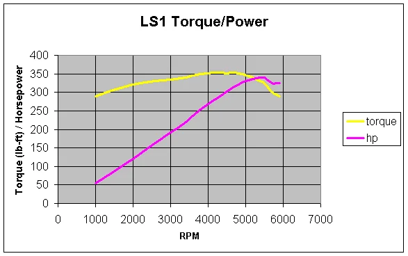
Now, a quickie: rpm (revolution per minute), basically how many times the engine made a full 360 degree spin with its shaft in 1 minute. In this context, we can think of the relationship between torque and rpm as follow:
Block
And by the way, we won’t be touching hp (horsepower) in pretty much our entire roadmap, its just an equivalent unit more commonly used amongst car folks and engineers.
Here’s the same plot using SI units, matching our current unit set:
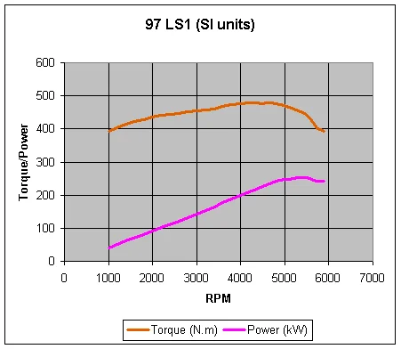
Again, we will only be focusing on torque, so pay attention to the orange line for now.
Now, as someone who have never driven before, when I first look at this, my first question is: “Why isn’t this orange line always increasing?”. Well, the engine basically have a “sweet-spot” for it to be able to deliver maximum torque, which is usually around the mid-high range of this line as you can see, once we go past that maxima, both torque and power goes down.
What’s more, notice how this plot isn’t defined at $ \leq 1000 $ rpm and $ ~> 6000 $ rpm, the specific value here doesn’t really matter, lets just call them the left side and the right side…
In car lingo, the left side is called the stall zone meaning you can’t really produce torque successfully at that rpm, again, we are not dealing with an arbitrary force generator anymore, we are dealing with a real life engine. Basically if you start an engine, it have to start spinning at that rpm. Not that it can’t literally spin at that rpm, but rather, it can’t maintain it without dying and needing to restart.
And beyond the right side, is what they call the redline, if you go beyond this point, you will damage your engine.
1.1.2. Example Torque Curve Implementation
But now, what does this curve actually mean for us? And what is its relation to the new $F_{drive}$ equation?
Having defined that $T_{engineMax} = f(rpm)$, and seeing that the torque curve doesn’t seem to be a function (these curves are determined from engine tests), we can imagine that we will be implementing this torque thing with a look up table, something like this:
# Simplified Torque Lookup Table for an LS1 Engine (RPM, Torque in Nm)
# Based on SI unit plot values
TORQUE_CURVE = [
    (1000, 390),
    (2000, 430),
    (3000, 450),
    (4000, 470),
    (4400, 475), # Peak Torque
    (5000, 460),
    (6000, 390)  # Redline
]

def get_max_torque(rpm):
    # Handle Stall Zone and Redline boundaries
    if rpm <= TORQUE_CURVE[0][0]: return TORQUE_CURVE[0][1]
    if rpm >= TORQUE_CURVE[-1][0]: return TORQUE_CURVE[-1][1]

    # Linear Interpolation between points
    for i in range(len(TORQUE_CURVE) - 1):
        rpm_low, torque_low = TORQUE_CURVE[i]
        rpm_high, torque_high = TORQUE_CURVE[i+1]

        if rpm_low <= rpm <= rpm_high:
            # Calculate how far we are between the two points (0.0 to 1.0)
            fraction = (rpm - rpm_low) / (rpm_high - rpm_low)
            return torque_low + fraction * (torque_high - torque_low)
    return 0
And for rpm, we can calculate it from the car’s current motion:
Block
where:
Block
1.1.3. Gear Selection
At this point, you might notice something:
- The torque curve is fixed
- But we multiply it by $ x_g $ So:
gears reshape how the torque curve appears at the wheels
We will now make that explicit.
GEARS = {
    1: 2.66,
    2: 1.78,
    3: 1.30,
    4: 1.00,
    5: 0.74,
    6: 0.50
}
So at any moment, the system is using:
Block
1.1.4. Stall Zone and Redline
Now, remember our stall zone? in implementation, we can do something like this:
rpm = max(rpm, rpm_idle) # rpm_idle ~1000
So technically, the engine is always running for our simulator. You may be asking, if the engine is spinning, and both rpm and torque is only defined starting from 1000 and below 6000, so meaning that we are idling with the engine spinning at 1000 rpm, so is my car going to always move? Well, for that, we are going to talk about a real pedal in a car called a clutch, its a component for the driver to disconnect the engine from the wheels, meaning the engine spins but the wheels doesn’t. We are going to talk more about it later, for now, don’t worry about that.
And about the redline, if we simply do:
rpm = min(rpm, rpm_redline)
then we aren’t actually simulating a “limit”, we are just pretending the engine stops getting faster while still allowing it to produce maximum force.
So instead, what we should do is:
if rpm > rpm_redline:
    T_engine = 0
above approach is called a rev limiter. This creates a “hard cut” where the engine stops producing torque until the RPM drops back into the safe zone. This provides immediate feedback to the player that they need to shift gears. If this gets confusing… it was and probably still is for me too, just kinda know that actual real cars does this rev limiter thing. In real car, say the engine is doing a smooth continuous “rvrrrrrrr”, this rev limiter thing is what make that “rvrm rvrm rvrm rvrm rvrm rvrm” sound, which exactly translate to us setting T_engine = 0 continuously as we are just neck close to the redline. (we approximate a rev limiter by cutting torque to zero intermittently, irl it doesnt really set torque to 0)
So thats $T_{engineMax}$ for us, but remember that the entire engine is:
Block
In the next section, we will be breaking down the rest of the arguments in the above equation.
1.2. Gear Ratios
In our drive force equation, $x_g$ (Gear Ratio) and $x_d$ (Differential Ratio) transform engine effort into wheel force. For a Corvette C5, the values look like this:
| Gear | Ratio ($x_g$) | Total Multiplier ($x_g \cdot x_d$) |
|---|---|---|
| First gear | 2.66 | ~9.10 |
| Second gear | 1.78 | ~6.08 |
| Third gear | 1.30 | ~4.44 |
| Fourth gear | 1.00 | ~3.42 |
| Fifth gear | 0.74 | ~2.53 |
| Sixth gear | 0.50 | ~1.71 |
| Reverse | 2.90 | ~9.91 |
| Differential | $x_d = 3.42$ | ___ |
Think of the Differential Ratio as a global multiplier that’s always on. The Gear Ratio is the one the driver (or your code) swaps out.
In 1st gear, your total multiplier is 9.1. This means for every $1\text{ Nm}$ of torque your engine makes, the axle gets $9.1\text{ Nm}$ of twisting force. Even if we lose 30% of that energy to heat and friction ($n = 0.7$), we still end up with a massive mechanical advantage.
1.2.1. Strength vs. Speed
You can’t just multiply torque forever and get a rocket ship for free. Physics demands a trade-off: Strength vs. Speed.
- Low Gears (High Ratio): You get massive torque (strength) to overcome the car’s inertia and start moving, but the engine has to spin 9.1 times just to make the wheels spin once.
- High Gears (Low Ratio): You get less torque, but the wheels can spin much faster relative to the engine. This is why you can’t start a car in 6th gear. You have the speed, but not the muscle to move the mass.
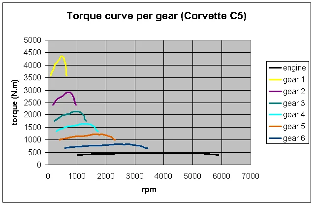
This is how it looks when we plot it. The yellow line (Gear 1) is a huge spike of torque, but it runs out of RPM very quickly. The dark blue line (Gear 6) is much lower, but it stretches way further to the right.
The above plot we looked at was technically correct, but it’s a bit confusing. It tells you what the motor is doing, but it doesn’t tell you what the car is doing. To bridge that gap, take a look at this plot:
Max Tractive Force - $F_{drive}$ (Gear 1): 12404 N
Theoretical Top Speed (Gear 6 @ 6000 RPM): 92.6 m/s (333 km/h)
- The X-Axis (Speed in m/s): Now, you can see exactly how much “road” each gear covers.
- The Y-Axis (Tractive Force in N): Instead of Torque (which is rotational), we are measuring Newtons. This is the direct translation for the tires exert against the asphalt to move the car’s mass forward.
The black dotted curve is the Optimal Envelope: for each speed it shows the maximum tractive force available across all gears. Staying on this envelope maximizes acceleration. Where two gear curves cross is the mathematical shift point, beyond that speed a higher gear produces more tractive force, so remaining in the lower gear would reduce acceleration.
1.2.2. The Final Calculation
To get the final $F_{drive}$ that we actually plug into our physics loop, we take that engine torque and finish the math:
Block
Using the Corvette example at peak torque ($475\text{ Nm}$) in 1st gear:
Block
With $9166\text{ N}$ of force pushing a $1439\text{ kg}$ car, you get an acceleration of $6.4\text{ m/s}^2$.
BlockNote: if you notice, some curves in the plot above are defined within the stall zone that we mentioned. Its crucial to know that X-axis on this specific plot isn’t representing Engine RPM (like in the torque power curve plot) anymore, it is representing Axle RPM (the speed of the rear wheels). Each gear maps engine RPM to a different vehicle speed range, which is why the curves stretch differently along the X-axis.
When you are in a high gear ratio (like 1st gear), the wheels spin much slower than the engine.
1.2.3. About the Clutch
Earlier, I briefly mentioned the clutch, to recap: Up until now, we’ve been assuming that the engine and the wheels are always perfectly connected. In reality, that’s not always true, and this is where the clutch comes in.
The clutch is a component that allows the driver to temporarily disconnect the engine from the drivetrain. When you press the clutch pedal, the engine can keep spinning freely without forcing the wheels to spin with it.
Now, for our simulator(s), we are not implementing the clutch (at least not until much later, probably). I think right now, it just adds way to much complexity and is genuinely a difficult component to grasp especially for people who have never driven before. This is not physically perfect, but it keeps the system stable, simple, and focused on the core ideas.
1.2.4. Transmission Modes Going Forward
“Transmission” just mean a connection between the engine and the wheels when talking about a car, it “transmits” power. With that being said, starting from model 3, I will be focusing on 2 main transmissions:
-
Manual transmission:
- You control gear shifting directly
- No clutch (so this is a simplified manual)
-
Automatic transmission:
- The system shifts gears for you
- Brake can also act as reverse at low speeds
This lets us explore the physics and behaviors without literally learning how to drive. Automatic will also be helpful if in the future we want to explore autonomous vehicles ;).
1.2.5. Extra Resources
I find the Youtube channel Sabin Civil Engineering extremely useful in understanding the engine in a manual transmission car:
More videos to learn about the:
- Footbrake:
- Handbrake:
2. The Suction Cup Wheels
You might have noticed something, it seems we have this loop:
engine torque -> wheel torque -> drive force -> car acceleration
 -> car speed -> wheel speed -> engine rpm -> engine torque
To compute engine torque, you need rpm. But rpm depends on wheel speed. And wheel speed depends on car speed. And car speed depends on engine torque. And our ambiguity here comes from this specific link: car speed -> wheel speed.
Let’s take a look at drive force again:
Block
And the torque curve:
Block
Earlier in Section 1.1.2., I seemingly brushed through these 2 formulas:
Block
where:
Block
And in $(*)$, that is exactly how we solve it for model 3. Let’s take that “loop” we mentioned and actually break it down into math (if the directionality is confusing you, just swap left hand side and right hand side):
- Engine torque <- Engine RPM
Block
Where $f$ is a lookup table (torque curve). $ 1 rpm = \frac{2 \pi}{60} rad/s $.
- Engine RPM <- Wheel Speed
Block
Where $\omega_{wheel}$ is the wheel speed, with unit $rad/s$.
- Wheel Speed <- Car Speed
Block
With:
| Variable | Unit |
|---|---|
| $ v $ | m/s |
| $\omega_{wheel}$ | rad/s |
| $ R_w $ (wheel radius) | m |
- Car Speed <- Car Acceleration
Block
- Car Acceleration <- Drive Force
Block
- Drive Force <- Wheel Torque
Block
- Wheel Torque <- Engine Torque
Block
And then we continue the cycle. If we want to be even more concise, we migth do:
Block
And, the key is here, because of $ (*) $, we implied that:
Block
This mean in model 3, our wheels have:
- No slip
- No lag
- No inertia
Or in other words, as if the wheels were glued to the ground, thus, the suction cup wheels.
In model 3, the wheel speed at its contact point with the ground must match the car speed this implies
- The contact patch never slips
- The ground has infinite grip
- Torque is always fully converted into forward motion
So if we were to get a bit more technical, model 3 is a velocity-dependent force system, not a realistic traction based one, yet.
This section doesn’t add new equations, but it exposes the key assumption that makes the engine model solvable.
3. Simulator 3 - Core Module
Let’s take a look at model 2’s core code module:
# === CONSTANTS (from Model 2) ===
g = 9.81
L = 2.8
h = 0.5
b = 1.7
c = 1.1


class CarModel:
    def __init__(self):
        self.x = 0.0
        self.v = 0.0

    def update(self, dt, u, B):

        # --- MODEL 1 PHYSICS ---
        F_engine = u * F_ENGINE_MAX
        F_rr = C_RR * self.v
        F_drag = C_DRAG * self.v * abs(self.v)
        F_brake = C_BRAKING if (self.v > 0 and B == 1) else 0

        F_net = F_engine - F_rr - F_drag - F_brake
        a = F_net / M

        self.v += dt * a
        if self.v < 0:
            self.v = 0

        self.x += dt * self.v


        # --- MODEL 2 DERIVED VALUES ---
        W = M * g
        dW = (h / L) * M * a

        Wf = (c / L) * W - dW
        Wr = (b / L) * W + dW

        return Wf, Wr
Up until Model 2, our “engine” was just a single line:
F_engine = u * F_ENGINE_MAX
In Model 3, we are not changing the physics loop itself. The structure:
force -> acceleration -> velocity -> position
stays exactly the same.
What we are doing instead is replacing that one line with a small subsystem:
v -> wheel speed -> rpm -> torque -> drive force
So conceptually:
OLD:
u -> F_engine

NEW:
u + v -> rpm -> T_engine -> F_drive
3.1. Actual Changes
Let’s look at the original Model 2 core again:
F_engine = u * F_ENGINE_MAX
This line is the only thing we remove.
Everything else: drag, rolling resistance, braking, integration, stays untouched.
3.2. New state variables
To support Model 3, we need to introduce a few new variables:
self.gear = 1
self.rpm = 1000  # idle rpm
(We don’t simulate clutch, at least not yet)
3.3. Reconstruct the pipeline
We now compute force in stages.
- Wheel angular velocity (suction cup wheels version)
omega_wheel = self.v / R_w
- Engine RPM
rpm = omega_wheel * x_g[self.gear] * x_d * 60 / (2 * math.pi)
rpm = max(rpm, RPM_IDLE)
- Torque from curve
T_engine_max = get_max_torque(rpm)
T_engine = u * T_engine_max
- Wheel torque
T_wheel = T_engine * x_g[self.gear] * x_d * eta
- Drive Force
And the final component:
F_engine = T_wheel / R_w
This is the direct replacement for the old:
F_engine = u * F_ENGINE_MAX
3.4. Full Updated Module
You can present it like this, only the engine part changed:
def update(self, dt, u, B):

    # --- MODEL 3 ENGINE SYSTEM ---

    omega_wheel = self.v / R_w

    rpm = omega_wheel * x_g[self.gear] * x_d * 60 / (2 * math.pi)
    rpm = max(rpm, RPM_IDLE)

    T_engine_max = get_max_torque(rpm)
    T_engine = u * T_engine_max

    T_wheel = T_engine * x_g[self.gear] * x_d * eta
    F_engine = T_wheel / R_w


    # --- SAME PHYSICS AS BEFORE ---

    F_rr = C_RR * self.v
    F_drag = C_DRAG * self.v * abs(self.v)
    F_brake = C_BRAKING if (self.v > 0 and B == 1) else 0

    F_net = F_engine - F_rr - F_drag - F_brake
    a = F_net / M

    self.v += dt * a
    if self.v < 0:
        self.v = 0

    self.x += dt * self.v


    # --- MODEL 2 STILL WORKS ---

    W = M * g
    dW = (h / L) * M * a

    Wf = (c / L) * W - dW
    Wr = (b / L) * W + dW

    return Wf, Wr
You might notice that while we introduced gears earlier, in this implementation they are still static:
self.gear = 1
and used here:
x_g[self.gear]
So right now, the car is effectively stuck in a single gear. The moment we allow self.gear to change dynamically:
- the same car speed can map to different RPMs
- the engine can stay in its “sweet spot”, the “black envelope”
- acceleration behavior changes dramatically
this is the extended full core module:
import math

# === CONSTANTS ===

# --- Physical constants ---
g = 9.81  # gravity (m/s^2)

# --- Vehicle parameters ---
M = 1439.0   # mass (kg)
L = 2.8      # wheelbase (m)
h = 0.5      # center of mass height (m)
b = 1.7      # distance from CG to rear axle (m)
c = 1.1      # distance from CG to front axle (m)

# --- Aerodynamics / resistance ---
C_RR = 12.5        # rolling resistance coefficient
C_DRAG = 0.4257    # aerodynamic drag coefficient

# --- Braking ---
C_BRAKING = 8000.0  # constant braking force (N)

# --- Drivetrain ---
R_w = 0.33   # wheel radius (m)
x_d = 3.42   # differential ratio
eta = 0.7    # drivetrain efficiency

# --- Gear ratios (1-5 only for now) ---
x_g = {
    1: 2.66,
    2: 1.78,
    3: 1.30,
    4: 1.00,
    5: 0.74
}

# --- Engine limits ---
RPM_IDLE = 1000
RPM_REDLINE = 6000

# --- Torque curve (RPM, Torque in Nm) ---
TORQUE_CURVE = [
    (1000, 390),
    (2000, 430),
    (3000, 450),
    (4000, 470),
    (4400, 475),  # peak
    (5000, 460),
    (6000, 390)
]


def get_max_torque(rpm):
    # Clamp to curve bounds
    if rpm <= TORQUE_CURVE[0][0]:
        return TORQUE_CURVE[0][1]
    if rpm >= TORQUE_CURVE[-1][0]:
        return TORQUE_CURVE[-1][1]

    # Linear interpolation
    for i in range(len(TORQUE_CURVE) - 1):
        rpm_low, torque_low = TORQUE_CURVE[i]
        rpm_high, torque_high = TORQUE_CURVE[i + 1]

        if rpm_low <= rpm <= rpm_high:
            t = (rpm - rpm_low) / (rpm_high - rpm_low)
            return torque_low + t * (torque_high - torque_low)

    return 0.0


# === MODEL ===

class CarModel:
    def __init__(self):
        self.x = 0.0
        self.v = 0.0

        # Model 3 additions
        self.gear = 1
        self.rpm = RPM_IDLE

    def update(self, dt, u, B):

        # --- MODEL 3 ENGINE SYSTEM ---

        # Wheel angular velocity (suction cup assumption)
        omega_wheel = self.v / R_w

        # Engine RPM from wheel speed
        rpm = omega_wheel * x_g[self.gear] * x_d * 60 / (2 * math.pi)
        rpm = max(rpm, RPM_IDLE)

        # Simple rev limiter (hard cut)
        if rpm > RPM_REDLINE:
            T_engine = 0.0
        else:
            T_engine_max = get_max_torque(rpm)
            T_engine = u * T_engine_max

        # Store for later use / debugging
        self.rpm = rpm

        # Drivetrain -> wheel torque -> force
        T_wheel = T_engine * x_g[self.gear] * x_d * eta
        F_engine = T_wheel / R_w

        # --- SAME PHYSICS AS BEFORE ---

        F_rr = C_RR * self.v
        F_drag = C_DRAG * self.v * abs(self.v)
        F_brake = C_BRAKING if (self.v > 0 and B == 1) else 0.0

        F_net = F_engine - F_rr - F_drag - F_brake
        a = F_net / M

        self.v += dt * a
        if self.v < 0:
            self.v = 0.0

        self.x += dt * self.v

        # --- MODEL 2 DERIVED VALUES (unchanged) ---

        W = M * g
        dW = (h / L) * M * a

        Wf = (c / L) * W - dW
        Wr = (b / L) * W + dW

        return Wf, Wr
In the next section, we’ll focus on making the controls more realistic by introducing gear shifting behavior (both manual and automatic).
4. Simulator 3 - Controls
We have been focusing on physics and engineering, now, is time to actually make our simulator 3.
4.1. Control Inputs
We keep the common input space minimal:
| Input | Meaning | Range |
|---|---|---|
| ( u ) | throttle | [0, 1] |
| ( B ) | brake | [0, 1] |
Compared to previous models, the key change is that braking is now analog, not binary.
Instead of:
F_brake = C_BRAKING if B == 1 else 0
we now have:
Block
In code:
if self.v != 0:
    F_brake = -B * C_BRAKING * math.copysign(1, self.v)
else:
    F_brake = 0.0
This will make the car have a smoother deceleration instead of on/off braking, helping us to control stopping distance and provide a more natural driving feel.
4.2. Manual Transmission
We start with a simplified manual transmission.
4.2.1. Core flow
The user directly shifts the gear:
if gear_up:
    self.gear = min(self.gear + 1, MAX_GEAR)

if gear_down:
    self.gear = max(self.gear - 1, MIN_GEAR)
4.2.2. What this implies
- shifting is instantaneous
- incorrect gear choice is allowed
- engine RPM is always derived from speed
This keeps the system consistent with:
Block
4.3. Automatic Transmission
Instead of direct control, we can let the system choose gears. Gears shifting help keep the engine in a reasonable RPM range.
4.3.1. Simple Shifting Logic
RPM_UPSHIFT = 5500
RPM_DOWNSHIFT = 1500

if self.rpm > RPM_UPSHIFT and self.gear < MAX_GEAR:
    self.gear += 1

elif self.rpm < RPM_DOWNSHIFT and self.gear > 1:
    self.gear -= 1
4.3.2. What this implies
- shift up near redline
- shift down near stall
- keep engine near its “usable” region
We can make shifting responsive to throttle:
- high throttle -> later upshifts
- low throttle -> earlier upshifts
This gives a more natural driving feel without adding much complexity.
4.4. Reverse Gear
This is a big one, starting from model 3, our car will be able to go in reverse. Reverse is handled differently from forward gears.
4.4.1. Key idea
Reverse is simply a negative gear ratio:
Block
4.4.2. Reverse in Manual Mode
Reverse can be treated as a special gear:
GEARS = [-1, 1, 2, 3, 4, 5]
The user shifts into it like any other gear.
4.4.3. Reverse in Automatic Mode
We can map inputs to direction, our brake will double up as going in reverse:
if abs(self.v) < v_threshold:
    if B > 0:
        self.gear = -1   # reverse
    elif u > 0:
        self.gear = 1    # forward
4.5. Safety Constraint and Assistive Features
4.5.1. Low Speed Braking Threshold
Reverse should only engage at low speed:
if abs(self.v) < 1.0:
    allow_reverse = True
Without this constraint, the model would allow instant direction flipping at high speed, presenting physically unrealistic behavior.
4.5.2. Idle Clamp
Again, to handle stalling:
rpm = max(rpm, RPM_IDLE)
4.5.3. Rev Limiter
And handle the redline:
if rpm > RPM_REDLINE:
    T_engine = 0
4.5.4. Near-zero Stabilization
if abs(self.v) < 0.1 and B > 0:
    self.v = 0.0
Prevents jitter when stopping.
5. Simulator 3 - Showcase
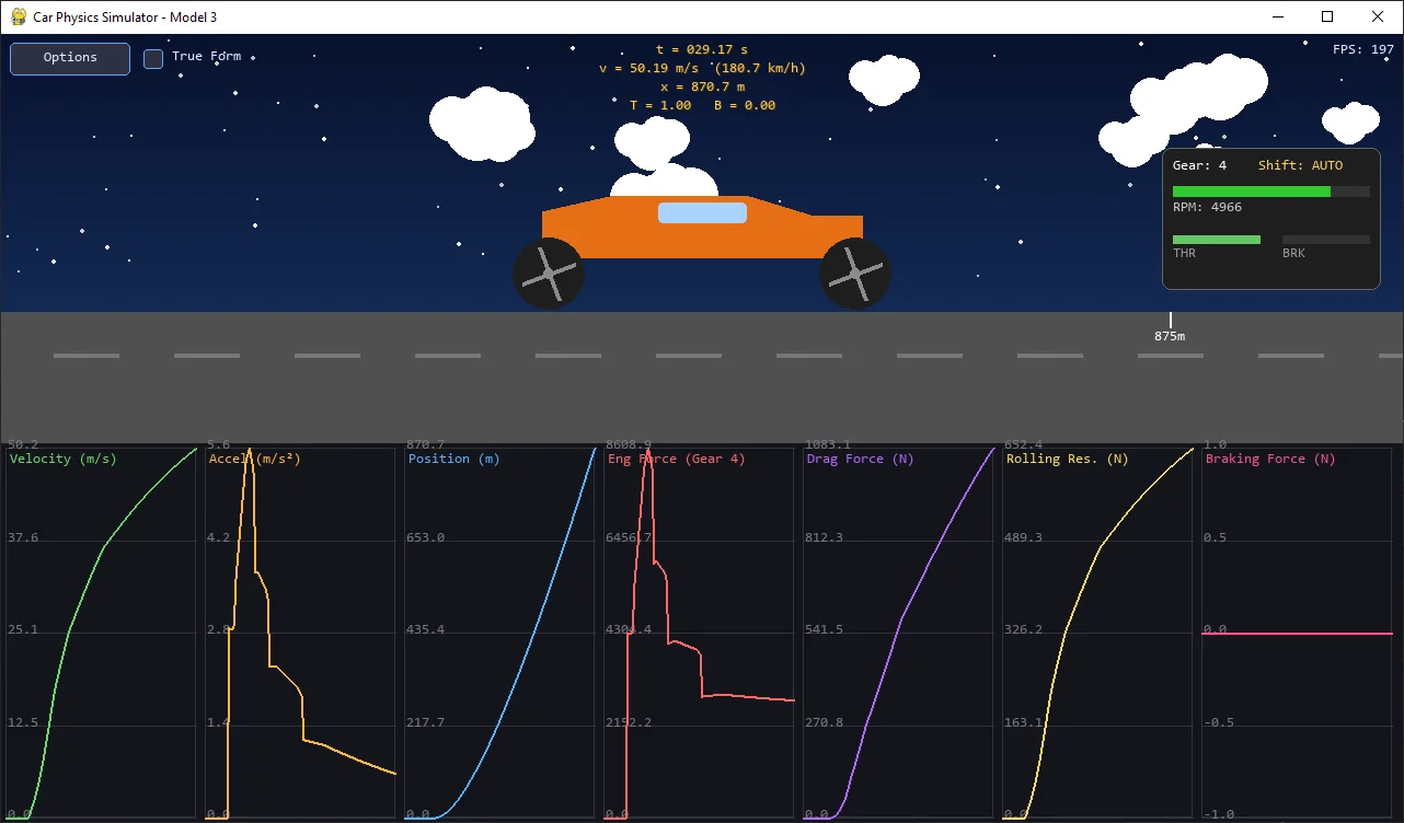
Also, because now we have wheel speed: $ \omega_{wheel} $, we can also give spinning animation to our wheels!
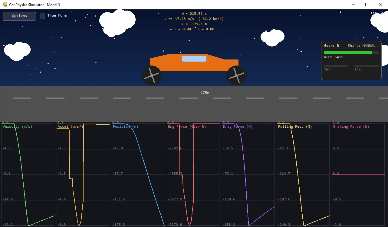
And thanks to the reverse gear, we can finally go in reverse in our simulator.
Check out the simulator at:
- Github repo for Longitudinal Simulators: duy-phamduc68/Longitudinal-Car-Physics
6. Final Takeaways
This section wraps up Model 3: Engine Torque + Gearing without Slip (1D) by summarizing what was added, what fundamentally changed, and what limitations still remain.
6.1. The Engine - Drivetrain Model
Model 3 replaces the artificial constant force with a physically grounded pipeline:
Block
Block
Block
And critically, engine RPM is no longer arbitrary:
Block
with:
Block
6.2. The Key Assumption: “Suction Cup Wheels”
To make this system solvable, Model 3 introduces a crucial constraint:
Block
This implies:
- no slip
- no wheel spin
- no wheel lock
- no independent wheel dynamics
In other words, wheel speed is fully determined by vehicle speed.
6.3. Actual Changes
Unlike Model 2, this is not just an added derived values, this changes the structure of the system.
Previously:
u -> force -> acceleration -> velocity
Now:
v -> rpm -> torque -> force -> acceleration -> v
This creates a closed loop where acceleration becomes a function of velocity
6.4. The Role of Gears
Gears introduce a discrete transformation into the system:
Block
They affect both:
- torque multiplication
- engine RPM
So instead of a single behavior, the engine now produces different force-speed profiles depending on the selected gear.
6.5. The Updated Implementation
The physics loop itself remains unchanged. Only the engine model is replaced.
# Core idea (simplified)

omega_wheel = v / R_w
rpm = omega_wheel * x_g[gear] * x_d * 60 / (2 * pi)

T_engine = u * f(rpm)
T_wheel = T_engine * x_g[gear] * x_d * eta

F_drive = T_wheel / R_w
Everything else:
- drag
- rolling resistance
- braking (becomes analog instead of binary)
- integration
remains identical to previous models.
You can revisit the full extended-updated implementation in 3.4. Full Updated Module.
6.6. Retrospective
Model 3 introduces:
- realistic torque curves
- meaningful gear ratios
- speed-dependent acceleration
- a proper engine-drivetrain pipeline
The car no longer behaves like a rocket, it behaves like a machine with internal structure.
Because of the suction cup assumption:
- no traction limits
- no slipping or skidding
- no wheel inertia
- no braking lock-up
So all forces are perfectly transmitted to the ground.
At this stage, the model is now clearly split into two layers:
- Physics layer:
engine -> drivetrain -> force -> motion
- Control layer:
inputs -> throttle / brake / gear -> physics
The next major limitation is clear: “we assume the tires can always apply whatever force we ask for”
In reality, this is not true.
In Model 4, we will begin addressing this by introducing wheel rotational dynamics, where:
- wheel speed becomes a state
- torque produces angular acceleration
- the constraint $ v = \omega R $ is removed
This is the first step toward modeling traction and slip, which will be fully explored in Model 5. For now, we will be soon tackling Model 4: Wheel Rotational Dynamics (1D), see you then :).