Table of Content

• Table of Content
• Roadmap
• Prologue
• A. Continuous Math Derivation
• 1. States
• 2. Mental Model
• 3. Forces
• 3.1. Traction
• 3.2. Resistance
• 3.3. Braking
• 3.4. Total (master ODE)
• 4. Constraint
• 5. Exploring the model
• 5.1 The force balance dashboard
• 5.2 Scenario walkthroughs
• 5.3 Derivable quantities
• B. Code Implementation
• 6. The discretization bridge
• 6.1. The core problem
• 6.2. Euler’s Method
• 6.3. Choosing timestep
• 6.4. The Core discrete update function (Pseudocode)
• 6.5. Side-by-Side: continuous vs. discrete
• 7. Simulator
• C. Final Takeaways
• 8. What Model 1 CAN Do
• 9. What Model 1 CAN’T Do

Block

• Main reference: Marco Monster’s Car Physics
• Github repo for Longitudinal Simulators: duy-phamduc68/Longitudinal-Car-Physics
• Github repo for Simulator 6: duy-phamduc68/Planar-Kinematic-Car-Model
• Github repo for Planar Dynamic Simulator(s): duy-phamduc68/Planar-Dynamic-Car-Model

Roadmap

• Model 1: Longitudinal Point Mass (1D)
  • Straight Line Physics
  • Magic Constants
  • Braking
• Model 2: Load Transfer Without Traction Limits (1D)
  • Weight Transfer
• Model 3: Engine Torque + Gearing without Slip (1D)
  • Engine Force
  • Gear Ratios
  • Drive Wheel Acceleration (simplified)
• Model 4: Wheel Rotational Dynamics (1D)
  • Drive Wheel Acceleration (full)
  • Torque on the Drive Wheel & The Chicken and The Egg
• Model 5: Slip Ratio + Traction Curve (1D)
  • Slip Ratio & Traction Force
• Model 6: Low-Speed Kinematic Turning (2D)
  • Curves (low speed)
• Model 7: High-Speed Lateral Tire Model (2D)
  • High Speed Turning
• Model 8: Full Coupled Tire Model (2D)

Block

Prologue

So recently after my new project TrafficLab 3D, beside my new found interest for simulation and digital twins, I’ve also got more into utilizing those environments themselves for something like autonomous driving. Moreover, I also sign up for a differential equations course this semester, so I thought might as well.

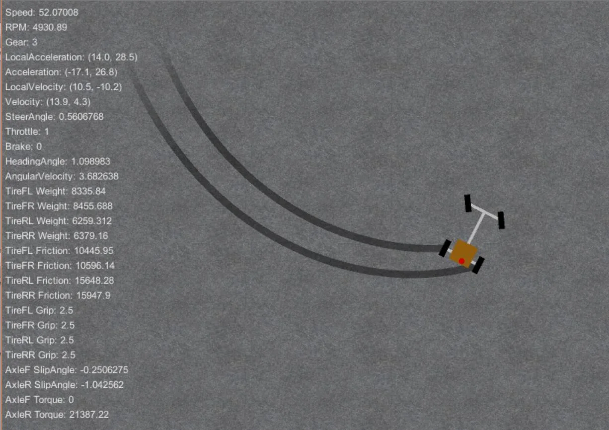
I’ve already scout what’s possible and pre-existing implementations, some cool stuff I found are:

• Car Demo.
• DanieloM83/R3F-Car-Racing.
• mattbradley/dash.
• TUMFTM/Open-Car-Dynamics.
• MetaDrive.

All is cool and all, but my end goal with this project is actually something like jongallant/CarSimulator. It seems simple enough, but also relevant to my current direction, particularly it resonates with my long-term goal of TrafficLab 3D (validating errors) and my new found interest for self-driving. Honestly, I was a bit worried that I might be doing less “AI” by taking up this project, but honestly, for self-driving car, most often time physics should come first before AI.

Anyway, jongallant/CarSimulator reference the Marco Monster’s Car Physics guide heavily, after reviewing both of them thoroughly, I find this challenge worthy to be tackled and eventually put on my portfolio. I plan to approach it from an educational standpoint first, which is why I’ve devise an 8 model roadmap, until I can achieve a complete implementation close to the one from jongallant. In this post, we will be deriving the very first model in the road map: Model 1: Longitudinal Point Mass (1D). I will assume a lot from the guide a lot so do have it on another tab or something.

A. Continuous Math Derivation

1. States

• $x(t) \geq 0$ : Position of the car. Meters (m).
• $v(t) = \frac{dx}{dt}$ : Velocity or the car. Meters per second (m/s).
• $a(t) = \frac{dv}{dt}$ : Acceleration of the car. Meters per second squared (m/s²).

2. Mental Model

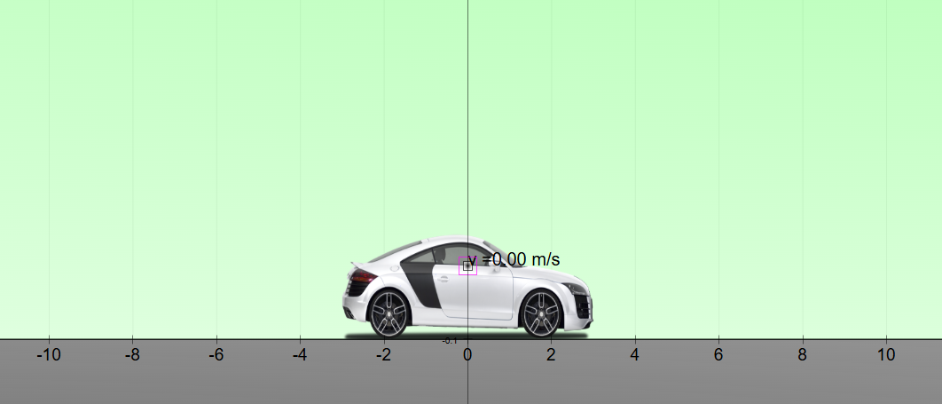
1D line, side profile of the car visible.

3. Forces

3.1. Traction

$$F_{\text{engine}} = u(t) \cdot F_{\text{engineMax}}$$

Block

Where:

• $u(t) \in [0,1]$ - Analog input.

3.2. Resistance

$$\begin{align*} F_{\text{resist}} &= F_{\text{rr}} + F_{\text{drag}} \\ &= C_{\text{rr}} \cdot v + C_{\text{drag}} \cdot v \cdot |v| \end{align*}$$

Block

Where:

• $F_{\text{rr}}$ : Rolling resistance (simplified - tires <-> road).
• $F_{\text{drag}}$ : Air resistance, a.k.a. aerodynamic drag (air <-> vehicle).

Magic constants:

$$C_{\text{drag}} = 0.5 \cdot C_d \cdot A \cdot \rho = 0.5 \cdot 0.30 \cdot 2.2 \cdot 1.29 \approx 0.4257$$

Block

Where:

• $C_d$ : Coefficient of friction, determined from wind tunnel tests. Here approximated to 0.30 reference for a Corvette.
• $A$ : Frontal area of the car, approx 2.2m² here.
• $\rho = 1.29$ kg/m³ : Air density.

$$C_{\text{rr}} \approx 30 \cdot C_{\text{drag}} \approx 12.8$$

Block

Very approximated.

3.3. Braking

Assumed a binary handbrake: $B(t) \in \{0, 1\}$.

$$F_{\text{braking}}(v, B) = \begin{cases} B \cdot C_{\text{braking}} & \text{if } v > 0 \\ 0 & \text{if } v = 0 \end{cases}$$

Block

3.4. Total (master ODE)

Remember Newton’s 2nd law: $ a = \frac{F}{m} $.

$$F_{\text{net}} = m \cdot a(t) = m \cdot \frac{dv}{dt} \\ \frac{dv}{dt} = \frac{1}{m} \left(F_{\text{engine}} - F_{\text{resist}} - F_{\text{braking}} \right)\\ \frac{dv}{dt} = \frac{1}{m} \left(u \cdot F_{\text{engineMax}} - \left(C_{\text{rr}} \cdot v + C_{\text{drag}} \cdot v \cdot |v| \right) - F_{\text{braking}}(B, v) \right)$$

Block

4. Constraint

For this model, we put this constraint for simplicity and preventing the car from going backwards:

$$\text{If } v = 0 \text{ and } \frac{dv}{dt} < 0, \text{ then set } \frac{dv}{dt} = 0$$

Block

it basically mean we can only accelerate, cruse, decelerate to stop, or hard stop, but we can’t go backwards, this might seem a pretty silly restriction, for video games, yeah its pretty silly, but I plan that we will approach going in reverse once we get to Model 3: Engine Torque + Gearing without Slip (1D), where we have an actual gear for going in reverse.

5. Exploring the model

Now that we have our Master ODE (ordinary differential equations), let’s interrogate it. In this section, we’ll translate the math back into driving experiences.

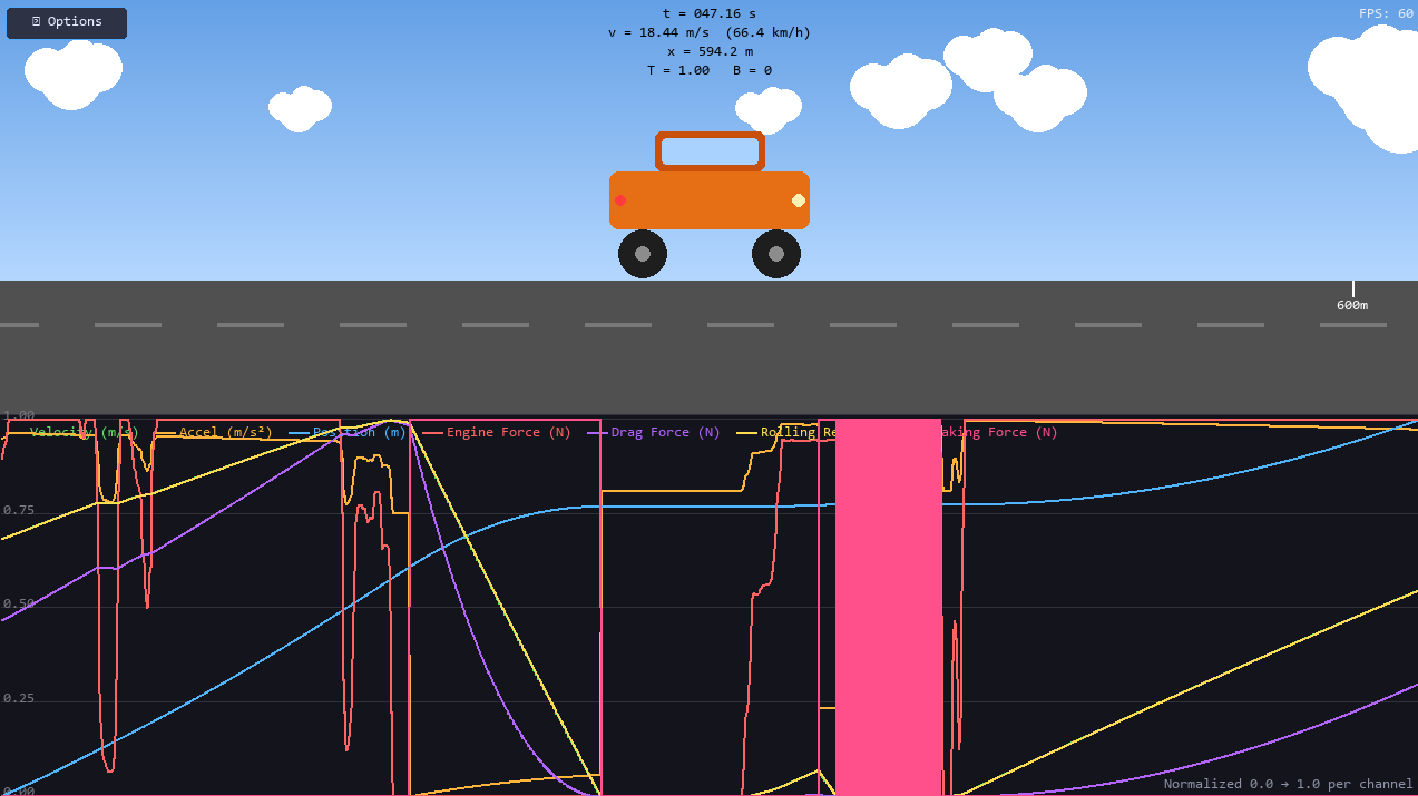
5.1 The force balance dashboard

The heart of Model 1 is the battle between propulsion and resistance. This dashboard lets you see that battle in real-time.

Note: these are just dummy stats, not from any real car:

M = 1500            # kg
F_ENGINE_MAX = 3000 # N
C_RR = 13.0         # kg/s
C_DRAG = 0.43       # kg/m
C_BRAKING = 12000   # N

Key insight: Reading equilibrium

The most important feature of this plot is the intersection point:

• Top speed occurs where Engine Force = Resistance Force.
• (i.e., where the Net Force line crosses zero)

Here are some intuitions you might want to walkthrough:

Mathematically, this is solving:

$$u \cdot F_{\text{engineMax}} = C_{\text{rr}} \cdot v_{max} + C_{\text{drag}} \cdot v_{max}^2$$

Block

You can solve this quadratic analytically (see Section 5.3), but the plot gives you an instant visual answer. Drag the throttle slider and watch the equilibrium point slide along the velocity axis.

On the same note, you can just see how simplified the braking here is. In reality, neither the handbrake nor the footbrake is binary, but instead analog. Also, a real car takes much longer to decelerate if you don’t plan for it, if you are zooming at top speed (in the dashboard above, say 70m/s $\approx$ 252km/h), don’t expect the car to stop sub-second or even in 2-3 seconds irl. This will be partially address in Model 2: Load Transfer Without Traction Limits (1D).

5.2 Scenario walkthroughs

The Master ODE is a compact statement, but it encodes many scenario in of itself. In this section, we’ll simulate specific scenarios and watch how the equation responds.

!Tips: Keep the Dashboard Open: Open Section 5.1 in another tab. We’ll reference it constantly.

Block

• Scenario 1: The Launch (Full Throttle from Stop)

Why? At $v=0$, both resistance terms vanish: $C_{rr} \cdot 0 = 0 \quad \text{and} \quad C_{drag} \cdot 0^2 = 0$ The engine fights only mass, not air or friction.

• Scenario 2: The Cruise (Top Speed Equilibrium)

Why? As speed increases, drag ($v^2$) grows rapidly. Eventually: $F_{max} = C_{rr} v_{max} + C_{drag} v_{max}^2$ The engine’s forward push is exactly canceled by air + road pushing back.

Analytical Bonus: Solve for $v_{max}$ directly: $v_{max} = \frac{-C_{rr} + \sqrt{C_{rr}^2 + 4 C_{drag} F_{engine}}}{2 C_{drag}}$ Plug in our constants: $v_{max} \approx 70 \, \text{m/s} \approx 252 \, \text{km/h}$.

• Scenario 3: The Coast (Lifting Off at Highway Speed)

Why? Drag scales with $v^2$. At 30 m/s: $F_{drag} = 0.43 \cdot 30^2 \approx 387 \, \text{N} \quad \text{vs} \quad F_{rr} = 13 \cdot 30 = 390 \, \text{N}$ They’re comparable here, but drag grows much faster as speed increases.

• Scenario 4: The Creep (Rolling to a Stop)

Why? At low $v$, the $v^2$ drag term becomes negligible: $C_{drag} \cdot 1^2 = 0.43 \, \text{N} \quad \text{vs} \quad C_{rr} \cdot 1 = 13 \, \text{N}$ Rolling resistance dominates, but it’s small → tiny deceleration.

The “Infinite Stop” Quirk: Because $F_{resist} \propto v$, as $v \to 0$, force $\to 0$. Mathematically, the car asymptotically approaches zero but never reaches it in finite time. In reality, static friction and our Hard Stop Constraint (Section 4) handle the final halt. We accept this trade-off for mathematical smoothness.

Block

• Scenario 5: The Hard Brake (Emergency Stop)

Why? The brake force ($12,000 \, \text{N}$) dwarfs resistance forces at most speeds. Deceleration is nearly constant until $v$ gets very low.

• Scenario 6: The Hard Stop (At Rest, Holding Brake)

Why? At $v=0$, braking force is defined as zero (it only opposes motion). The constraint (Section 4) prevents the car from accelerating backward due to any residual negative force.

Quick Reference: Scenario <-> Dominant Term

5.3 Derivable quantities

One of the most satisfying aspects of having a formal ODE is that you can calculate exact answers without running a simulation.

In this section, we’ll derive a few key performance metrics directly from the Master ODE:

Why This Matters: These formulas let you tune your car analytically. Want a 10% faster top speed? The equations tell you exactly how much to increase engine force or reduce drag.

Block

Derivable 1: Top Speed

The Question: What is the maximum speed achievable at full throttle?

The Insight: At top speed, acceleration is zero ($\frac{dv}{dt} = 0$). The engine force exactly balances resistance.

Derivation:

$$\begin{align*} 0 &= \frac{1}{m} \left( F_{engine} - C_{rr} v_{max} - C_{drag} v_{max}^2 \right) \\ F_{engine} &= C_{rr} v_{max} + C_{drag} v_{max}^2 \\ C_{drag} v_{max}^2 + C_{rr} v_{max} - F_{engine} &= 0 \end{align*}$$

Block

This is a quadratic equation $ax^2 + bx + c = 0$ with:

• $a = C_{drag}$
• $b = C_{rr}$
• $c = -F_{engine}$

Solution (positive root only, since $v \ge 0$):

$$\boxed{ v_{max} = \frac{-C_{rr} + \sqrt{C_{rr}^2 + 4 C_{drag} F_{engine}}}{2 C_{drag}} }$$

Block

Interactive Calculator:

Key Insight: Top speed depends on the square root of engine force but only linearly on drag reduction.

Derivable 2: 0 to 100 km/h Time

The Question: How long does it take to accelerate from rest to 100 km/h (27.8 m/s)?

The Insight: Time is the integral of “inverse acceleration” over velocity.

Derivation:

$$\begin{align*} a &= \frac{dv}{dt} \quad \Rightarrow \quad dt = \frac{dv}{a(v)} \\ t_{0-100} &= \int_{0}^{27.8} \frac{1}{a(v)} \, dv = \int_{0}^{27.8} \frac{m}{F_{engine} - C_{rr}v - C_{drag}v^2} \, dv \end{align*}$$

Block

The Challenge: This integral has no simple closed form (it involves $\arctan$ or $\ln$ depending on the discriminant). But we can evaluate it numerically for display.

Interactive Visualization:

Why Mass Matters Here: Unlike top speed, acceleration time does depend on mass. Heavier cars have smaller $a = F/m$, so the integral takes longer to accumulate. Try This: Double the mass in the code ($m = 3000$). The 0→100 time roughly doubles (not exactly, because resistance forces don’t scale with mass).

Derivable 3: Stopping Distance

The Question: How far does the car travel when braking hard from speed $v_0$ to rest?

The Insight: Use the chain rule trick: $a = v \frac{dv}{dx} \Rightarrow dx = \frac{v}{a(v)} dv$.

Derivation:

$$\begin{align*} a &= \frac{dv}{dt} = \frac{dv}{dx} \cdot \frac{dx}{dt} = v \frac{dv}{dx} \\ \Rightarrow \quad dx &= \frac{v}{a(v)} dv \\ d_{stop} &= \int_{v_0}^{0} \frac{v}{a(v)} dv = \int_{0}^{v_0} \frac{m \cdot v}{C_{braking} + C_{rr}v + C_{drag}v^2} dv \end{align*}$$

Block

Note: The limits flip because we’re integrating from high speed to zero, but distance is positive.

Interactive Calculator:

Key Insight: Stopping distance scales roughly with $v_0^2$ (because kinetic energy is $\frac{1}{2}mv^2$). Doubling your speed quadruples your stopping distance.

Mass Matters: Unlike top speed, stopping distance increases with mass because $d \propto m$ in the integral. Heavier cars take longer to stop.

Summary: What You Can Calculate Analytically

B. Code Implementation

Now that we have a solid mental model of the continuous mathematics, we need to bridge the gap to discrete computation.

6. The discretization bridge

6.1. The core problem

Our Master ODE describes instantaneous change:

$$\frac{dv}{dt} = \frac{1}{m} \left( F_{engine} - F_{resist} - F_{braking}(v, B) \right)$$

Block

The term $\frac{dv}{dt}$ is a derivative, it asks: “What is the rate of change at this exact instant?”

Computers cannot compute “instants.” They compute steps. We need to approximate the continuous derivative using discrete time intervals.

6.2. Euler’s Method

The simplest discretization is Forward Euler Integration, if you are familiar with implementing a neural network from scratch, particularly, Gradient Descent in code, then its very similar. Here’s the derivation:

• Step 1: Start with the derivative definition

$$\frac{dv}{dt} \approx \frac{v_{new} - v_{old}}{\Delta t}$$

Block

Where $\Delta t$ (often written as dt) is the time step between updates.

• Step 2: Substitute the ODE

$$\frac{v_{new} - v_{old}}{\Delta t} = \frac{1}{m} F_{net}(v_{old})$$

Block

• Step 3: Solve for $v_{new}$

$$v_{new} = v_{old} + \Delta t \cdot \frac{F_{net}(v_{old})}{m}$$

Block

• Step 4: Similarly for position

$$x_{new} = x_{old} + \Delta t \cdot v_{old}$$

Block

The derivative $\frac{dv}{dt}$ becomes a finite difference $\frac{\Delta v}{\Delta t}$. We’re approximating the slope over a tiny interval instead of at an exact point.

Block

6.3. Choosing timestep

The timestep is a trade-off between accuracy and performance:

6.4. The Core discrete update function (Pseudocode)

Here’s the Master ODE translated into discrete steps:

# === CONSTANTS (from Model 1) ===
M = 1500            # kg
F_ENGINE_MAX = 3000 # N
C_RR = 13.0         # kg/s
C_DRAG = 0.43       # kg/m
C_BRAKING = 12000   # N


class CarModel:
    def __init__(self):
        # === STATE ===
        self.x = 0.0  # position (m)
        self.v = 0.0  # velocity (m/s)

    def update(self, dt, u, B):
        """
        dt : timestep (seconds)
        u  : throttle [0, 1]
        B  : brake [0, 1] (binary)
        """

        # 1. Calculate Forces
        F_engine = u * F_ENGINE_MAX
        F_rr = C_RR * self.v
        F_drag = C_DRAG * self.v * abs(self.v)
        F_brake = C_BRAKING if (self.v > 0 and B == 1) else 0

        # 2. Net Force
        F_net = F_engine - F_rr - F_drag - F_brake

        # 3. Acceleration (Newton's 2nd Law)
        a = F_net / M

        # 4. Integrate Velocity
        self.v = self.v + dt * a

        # 5. Apply Hard Stop Constraint
        if self.v < 0:
            self.v = 0

        # 6. Integrate Position
        self.x = self.x + dt * self.v

6.5. Side-by-Side: continuous vs. discrete

7. Simulator

Now after all of that, I built a simulator in Python for Model 1, you can check out the code at duy-phamduc68/Longitudinal-Car-Physics.

C. Final Takeaways

This section wraps up Model 1: Longitudinal Point Mass (1D) with a concise recap of what we built, what it can (and can’t) do, and where we’re heading next.

The Master ODE (Continuous Math)

$$\boxed{ \frac{dv}{dt} = \frac{1}{m} \left( u \cdot F_{max} - B \cdot C_{braking} - C_{rr} v - C_{drag} v^2 \right) }$$

Block

Subject to constraint: If $v = 0$ and $\frac{dv}{dt} < 0$, then $\frac{dv}{dt} = 0$.

The Core update function

# === CONSTANTS (from Model 1) ===
M = 1500            # kg
F_ENGINE_MAX = 3000 # N
C_RR = 13.0         # kg/s
C_DRAG = 0.43       # kg/m
C_BRAKING = 12000   # N


class CarModel:
    def __init__(self):
        # === STATE ===
        self.x = 0.0  # position (m)
        self.v = 0.0  # velocity (m/s)

    def update(self, dt, u, B):
        """
        dt : timestep (seconds)
        u  : throttle [0, 1]
        B  : brake [0, 1] (binary)
        """

        # 1. Calculate Forces
        F_engine = u * F_ENGINE_MAX
        F_rr = C_RR * self.v
        F_drag = C_DRAG * self.v * abs(self.v)
        F_brake = C_BRAKING if (self.v > 0 and B == 1) else 0

        # 2. Net Force
        F_net = F_engine - F_rr - F_drag - F_brake

        # 3. Acceleration (Newton's 2nd Law)
        a = F_net / M

        # 4. Integrate Velocity
        self.v = self.v + dt * a

        # 5. Apply Hard Stop Constraint
        if self.v < 0:
            self.v = 0

        # 6. Integrate Position
        self.x = self.x + dt * self.v

8. What Model 1 CAN Do

9. What Model 1 CAN’T Do

If it helps, model 1 behaves more like a rocket or a boat than an actual car. Whats more, the car in the simulator is a lie, this model act as if its a single point, with mass, acted upon by forces, in a 1D environment, hence, “Longitudinal Point Mass”.

If you spot any mistake or have any suggestions, please let me know! See you in Model 2: Load Transfer Without Traction Limits (1D) :).