Table of Content

• Table of Content
• Motivation
• The Problem Context
• System Overview
• The G Projection
• Phase 1 - Undistort
• Phase 2 - Homography
• Phase 3 - Parallax
• Metric Scale and Layout Alignment
• The X Engine
• Phase 1 - Perception
• Phase 2 - Projection & Geometry
• Phase 3 - Reconstruction
• TrafficLab 3D - The Application
• Qualitative Analysis
• What Remains Open
• Closing Remarks
• References

Block

• Github Repo: duy-phamduc68/TrafficLab-3D
• Full Academic Report: Google Drive
• Video Demo: TrafficLab 3D v1.0 Demo
• Setup Guide: TrafficLab 3D Guide

Motivation

This project started as a midterm report for an Advanced Computer Vision course, framed around the question of whether you could build a Digital Twin for Hanoi’s traffic using only monocular CCTV footage and a satellite image. The academic title was “Towards Building a Digital Twin for Hanoi’s Traffic System”. By the time the codebase was finalized and made public, the Hanoi-specific framing had been replaced by something more general: TrafficLab 3D - a standalone proof-of-concept that anyone can run on their own CCTV footage, for any flat location they can find on Google Maps.

This post documents the technical substance behind that transition. The motivation, the geometry, the pipeline, and the things that did not quite work the way they were supposed to.

The core premise is this: given an mp4 clip from a CCTV camera and a satellite screenshot of the same location, can we reconstruct a 3D scene - placing road users on a map with realistic orientation and speed - without any camera calibration data, LiDAR, or stereo setup? The answer is a qualified yes, and the qualifications are interesting.

The Problem Context

It helps to understand what kind of traffic this was originally designed for.

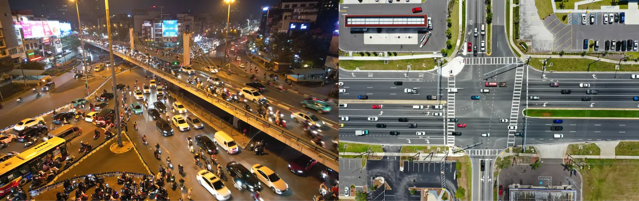
Left: Nga Tu So intersection, Hanoi. Right: New Port Richey, Florida. The domain gap is obvious.

Western computer vision datasets - COCO, KITTI, even most drone datasets - are built around structured, lane-disciplined traffic. Hanoi’s traffic is genuinely different. Two-wheelers dominate, they fill every gap, they do not respect lane geometry in the conventional sense, and the ontology of road users extends well beyond “car, bus, truck.” Three-wheelers, cargo motorbikes, and street vendor carts are common actors. The city’s infrastructure is also layered - overpasses, underpasses, and ring roads mean a single 2D projection is often insufficient even for flat intersections, let alone complex nodes.

Off-the-shelf models from 3D-Net (Rezaei et al., 2023), the main architectural inspiration here, failed for two concrete reasons when applied to this context. Their detection backbone was trained on MIO-TCD, a heavily Western-centric dataset with no motorcycle class to speak of. And their automated projection module - SG-IPM - relies on background subtraction to isolate road features. In Hanoi, the road is never empty. Background subtraction produces nothing useful when your “background” is continuously covered by a dense, moving foreground.

So both the detection and the calibration components needed to be rebuilt from scratch. That is what the $G$ Projection and the $X$ Engine are.

System Overview

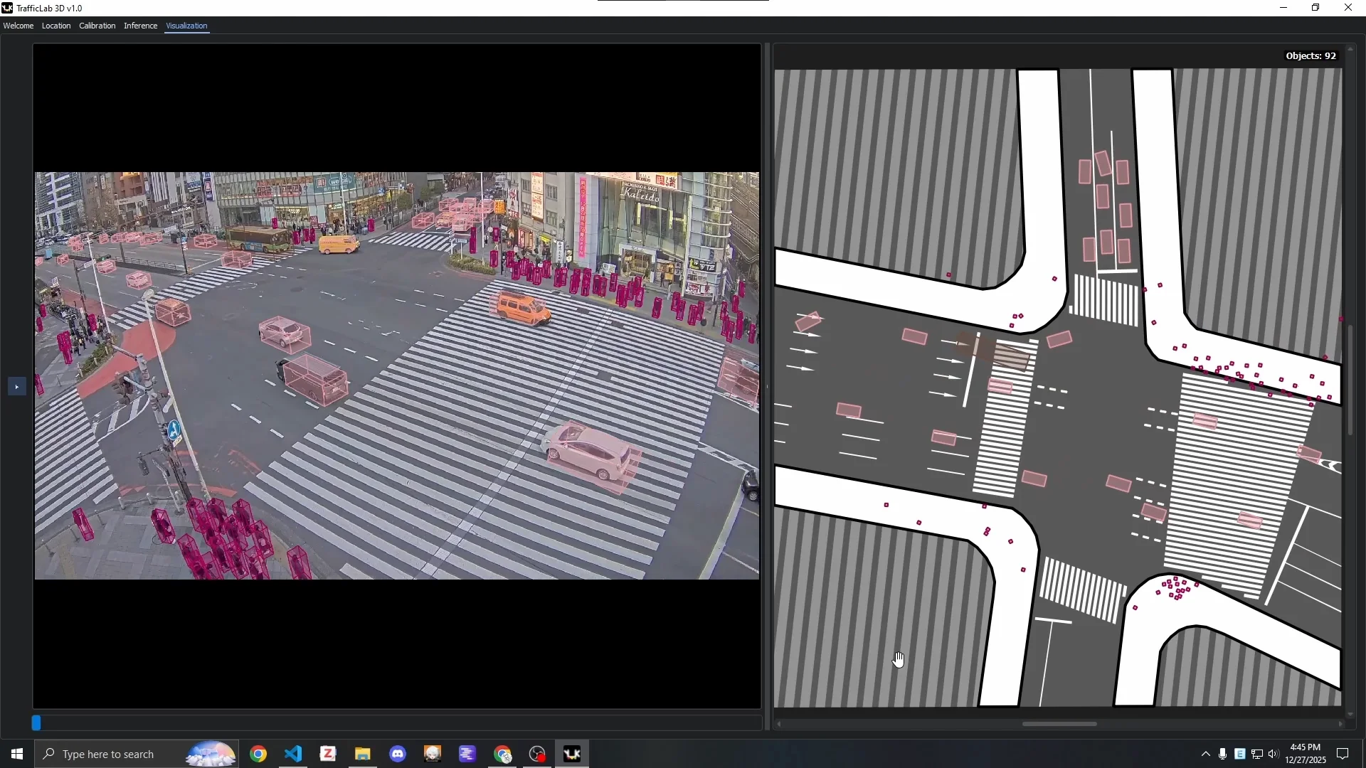
TrafficLab’s output is a synchronized, side-by-side visualization: the CCTV panel showing 3D bounding boxes in perspective, and the satellite panel showing orientation-aware floor boxes on the map with speed labels.

The system is organized around two core technical contributions:

• $G$ Projection: A dual mapping between CCTV image coordinates and satellite map coordinates, accounting for lens distortion and the parallax shift that comes from objects having non-zero height.
• $X$ Engine: A ten-step pipeline that uses the $G$ Projection to convert detected and tracked 2D bounding boxes into 3D reconstructions.

Everything is stored in JSON format and visualized through a PyQt5 GUI - now refactored into the TrafficLab 3D codebase with a full calibration tab, inference tab, and visualization tab.

The G Projection

The $G$ Projection is the geometric foundation of the whole system. It is a bidirectional mapping:

$$G_1 : (u, v, h)_{CCTV} \rightarrow (x, y)_{SAT}$$

Block

$$G_2 : (x, y, h)_{SAT} \rightarrow (u, v)_{CCTV}$$

Block

Here $(u, v)$ are pixel coordinates in the camera image, $(x, y)$ are pixel coordinates in the satellite image, and $h$ is a height parameter in meters. The presence of $h$ is what separates this from a simple homography - it is what allows us to project the top of a vehicle to a different location than its feet, which is the source of parallax error in perspective cameras.

Constructing a $G$ Projection for a location requires three inputs: a CCTV screenshot, a satellite screenshot, and optionally an SVG layout of the road geometry. The construction proceeds through three sequential phases.

Phase 1 - Undistort

Before anything else, raw CCTV pixel coordinates need to be rectified. CCTV lenses introduce distortion, most commonly the barrel distortion that curves straight lines. We adopt the standard pinhole model with Brown-Conrady radial-tangential distortion.

The intrinsic matrix is:

$$K = \left[ \begin{array}{ccc} f_x & 0 & c_x \\ 0 & f_y & c_y \\ 0 & 0 & 1 \end{array} \right]$$

Block

Given distorted pixel coordinates $(u, v)$, the normalized distorted coordinates are:

$$x_d = \frac{u - c_x}{f_x}, \qquad y_d = \frac{v - c_y}{f_y}$$

Block

The Brown-Conrady model maps undistorted normalized coordinates $(x_u, y_u)$ to the distorted ones via:

$$x_d = x_u(1 + k_1 r^2 + k_2 r^4 + k_3 r^6) + 2p_1 x_u y_u + p_2(r^2 + 2x_u^2)$$

Block

$$y_d = y_u(1 + k_1 r^2 + k_2 r^4 + k_3 r^6) + p_1(r^2 + 2y_u^2) + 2p_2 x_u y_u$$

Block

where $r^2 = x_u^2 + y_u^2$. The inverse - going from $(x_d, y_d)$ back to $(x_u, y_u)$ - has no closed form and is solved numerically. Rectified pixel coordinates are then:

$$u' = f_x x_u + c_x, \qquad v' = f_y y_u + c_y$$

Block

We define the undistortion operator $U : (u, v) \mapsto (u’, v’)$. All subsequent geometry operates on these rectified coordinates. In practice, since we have no camera spec sheet, all five distortion coefficients plus the intrinsics are adjusted manually in the calibration GUI, with a grid overlay to help judge when straight lines in the scene look straight.

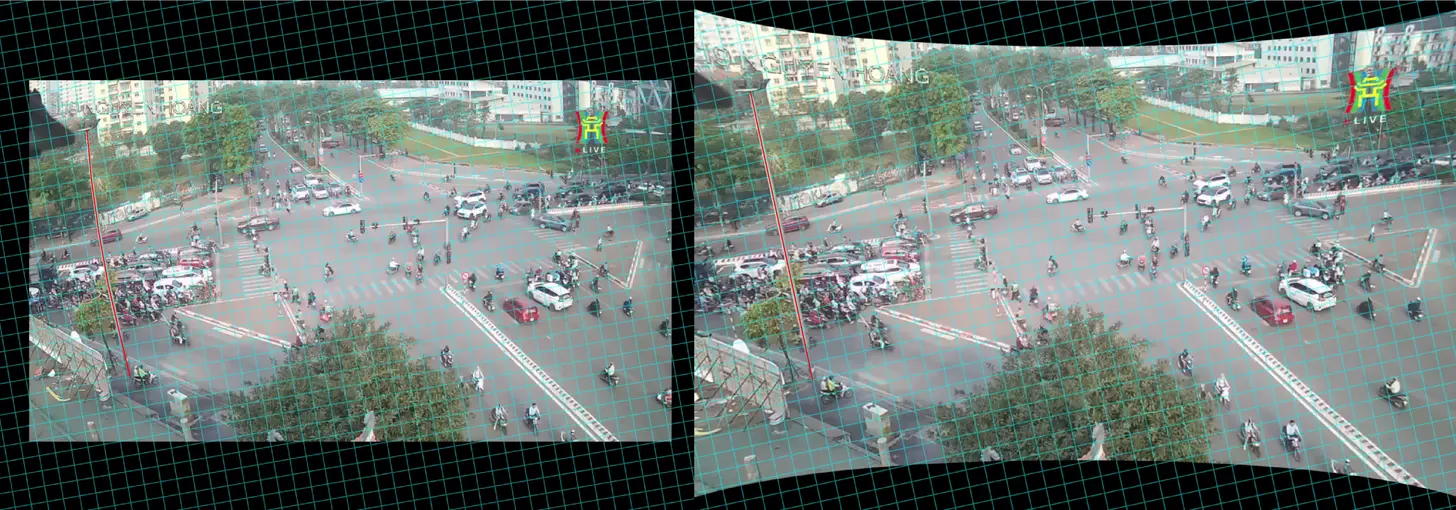
Undistortion for location 119NH. The pole on the left of the frame is used as a straightness reference.

Phase 2 - Homography

With rectified coordinates $(u’, v’)$, we now establish the mapping to the satellite image, under the assumption that everything is on the ground plane ($h = 0$). This is the classical homography problem.

Homography Definition

The homography $H$ maps a rectified CCTV point to a SAT point via homogeneous coordinates:

$$\left[ \begin{array}{c} x \\ y \\ 1 \end{array} \right] \sim \left[ \begin{array}{ccc} h_{11} & h_{12} & h_{13} \\ h_{21} & h_{22} & h_{23} \\ h_{31} & h_{32} & h_{33} \end{array} \right] \left[ \begin{array}{c} u' \\ v' \\ 1 \end{array} \right]$$

Block

Fixing $h_{33} = 1$ leaves 8 unknowns. Each correspondence pair $(u’_i, v’_i) \leftrightarrow (x_i, y_i)$ contributes two linear equations. Stacking these over the anchor set gives:

$$A h = b$$

Block

where each row pair of $A$ has the form:

$$A_i = \left[ \begin{array}{cccccccc} u'_i & v'_i & 1 & 0 & 0 & 0 & -x_i u'_i & -x_i v'_i \\ 0 & 0 & 0 & u'_i & v'_i & 1 & -y_i u'_i & -y_i v'_i \end{array} \right], \\ b_i = \left[ \begin{array}{c} x_i \\ y_i \end{array} \right]$$

Block

RANSAC Computation

Four correspondences are theoretically sufficient, but manual clicking introduces noise. In practice, we collect 10–12 anchor pairs at identifiable landmarks visible in both the CCTV and satellite frames - road markings, curb corners, traffic islands. We then use RANSAC to compute $H$ robustly:

1. Sample 4 random pairs, compute a candidate $H_{candidate}$.
2. Project all remaining points; count inliers where projection error is below a threshold (5px).
3. Repeat for a fixed number of iterations; keep the $H$ with the most inliers.
4. Refit $H$ using all inliers via least-squares.

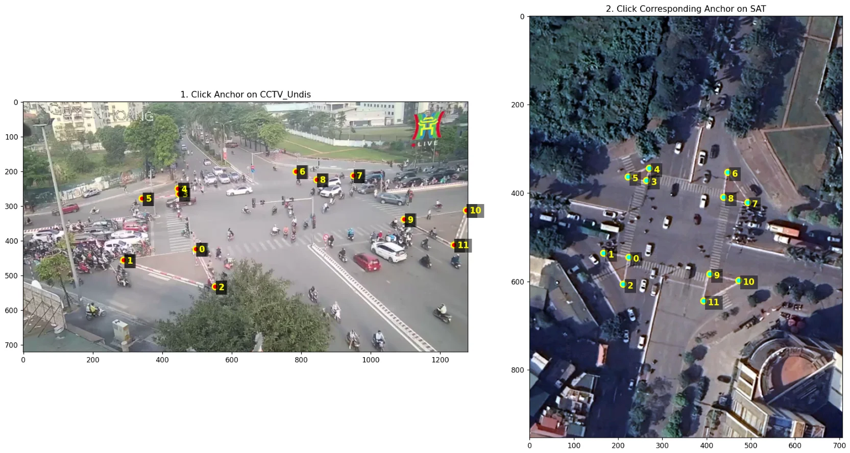
Anchor selection for 119NH. Left: points on the undistorted CCTV frame. Right: corresponding points on the satellite image.

Once $H$ is computed, we validate by warping the entire CCTV frame into satellite space and overlaying it on the satellite image. This also gives us the Field-of-View polygon - the observable area on the map.

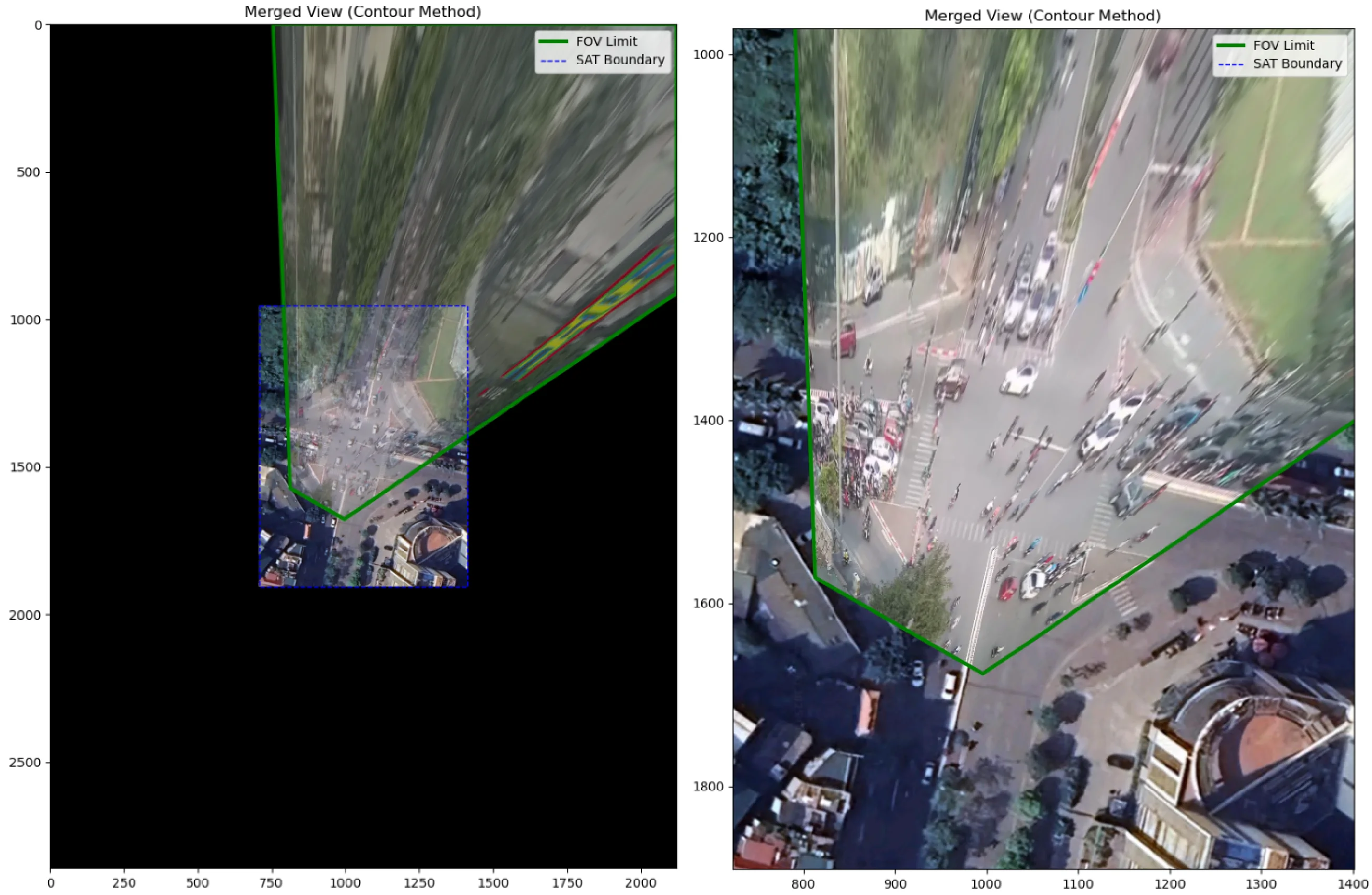
The green contour is the FOV limit. The warped CCTV image aligns with road edges and lane markings in the satellite view.

Bidirectionality

Since $H$ is a non-singular $3 \times 3$ matrix, its inverse exists and gives us the reverse direction:

$$\mathbf{p}_{sat} \sim H \mathbf{p}_{cctv}, \qquad \mathbf{p}_{cctv} \sim H^{-1} \mathbf{p}_{sat}$$

Block

At the end of Phase 2, we have $G : (u, v, 0) \leftrightarrow (x, y)$ - a working projection for ground-plane points only. Objects with height will be incorrectly placed on the satellite map, displaced away from their true position in the direction of the camera. That is the parallax problem Phase 3 solves.

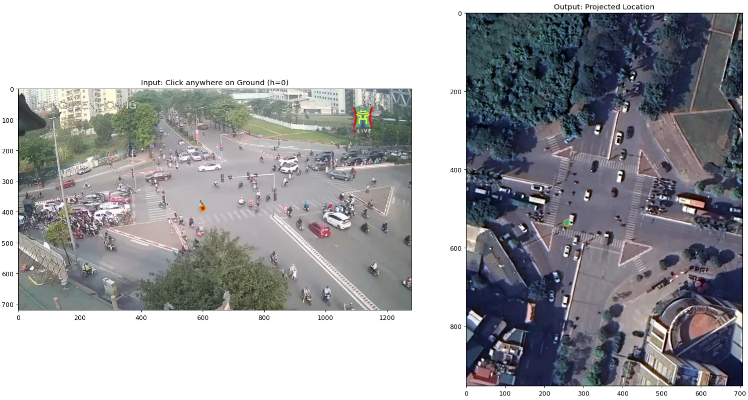
Demonstrating $G$ with $h=0$: a red marker in CCTV resolves to the aqua marker in SAT, and vice versa.

Phase 3 - Parallax

Consider what happens when you project the top of someone’s head using the ground-plane homography $H$. The head appears displaced from the feet in the camera image, so $H$ will map it to a different location on the satellite - “ghosted” toward the distance. This ghosting is the parallax shift, and it is proportional to height.

To undo it, we need to know where the camera is relative to the map. That is what Phase 3 computes.

Camera Localization via Parallax Rays

The key insight is that the ghosted projection of any vertical line points directly toward the camera’s optical center on the satellite map. Each “parallax ray” drawn from the true foot location through the apparent head location points to the same convergence point: the camera.

We select two reference subjects - specifically motorcycle riders - and assume a reference height $h_{ref} = 1.6\text{m}$. For each subject, we mark their head and feet in the undistorted CCTV image. We project both using $H$ into the satellite domain, which gives us:

• The feet → True Location $P_{feet}$
• The head → Apparent Location $P_{head}$

Drawing a line through $P_{feet}$ and $P_{head}$ for each subject, and intersecting those two lines, gives the camera’s satellite coordinates $C_{sat} = (X_{cam}, Y_{cam})$.

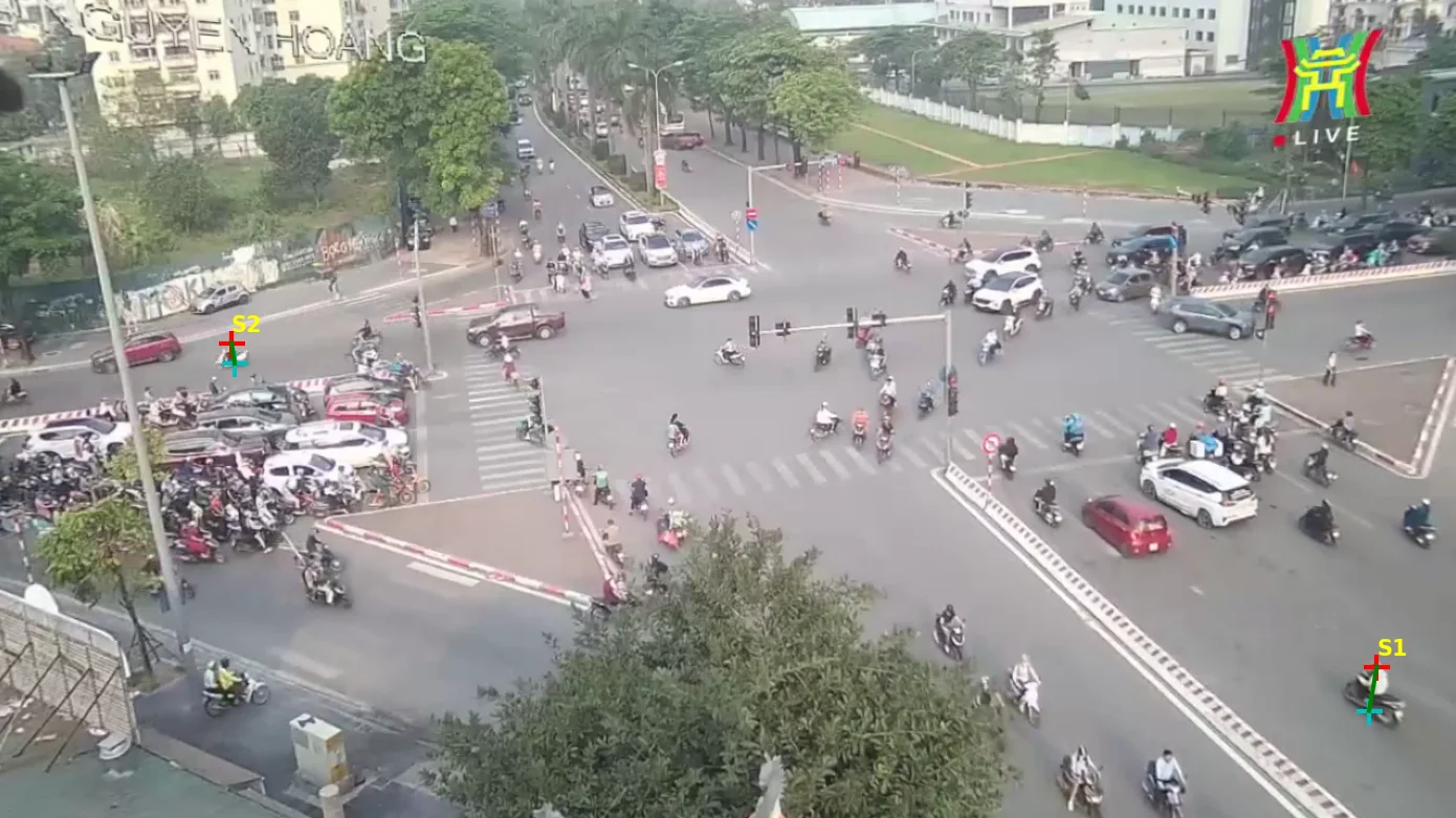
Two riders ($S_1$, $S_2$) with head (red) and feet (aqua) marked for parallax computation.

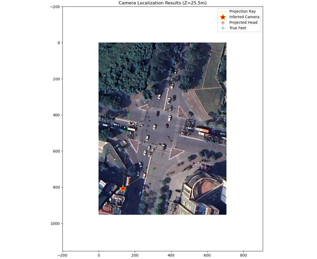
The yellow parallax rays intersect at the inferred camera position (red star) on the satellite map.

Camera Height

With the 2D camera position $C_{sat}$ known, we recover the camera’s altitude $Z_{cam}$ using similar triangles. The ratio of the parallax shift to object height is governed by the camera’s height:

$$Z_{cam} = \frac{h_{ref}}{1 - \dfrac{d_{true}}{d_{apparent}}}$$

Block

where $d_{true} = | P_{feet} - C_{sat} |$ and $d_{apparent} = | P_{head} - C_{sat} |$ are Euclidean distances in the satellite plane. This is computed for both reference subjects and averaged.

The General $G$ Projection

With the full camera geometry $(X_{cam}, Y_{cam}, Z_{cam})$ solved, we define the two directional mappings formally.

Localization ($G_1$): Given a CCTV pixel $(u, v)$ representing the top of an object at height $h$, we project with $H$ to get the apparent location $P_{apparent}$, then apply the parallax correction:

$$P_{true} = C_{sat} + (P_{apparent} - C_{sat}) \cdot \frac{Z_{cam} - h}{Z_{cam}}$$

Block

$$G_1(u, v, h) = P_{true}$$

Block

Reprojection ($G_2$): Given a true satellite location $(x, y)$ and height $h$, we first compute the apparent position by inverting the parallax ratio:

$$P_{apparent} = C_{sat} + ((x, y) - C_{sat}) \cdot \frac{Z_{cam}}{Z_{cam} - h}$$

Block

Then we map back to CCTV with the inverse homography:

$$(u, v) \sim H^{-1} P_{apparent}, \qquad G_2(x, y, h) = (u, v)$$

Block

These two functions are the engine. $G_1$ locates objects on the map, $G_2$ reconstructs their 3D bounding boxes in video space.

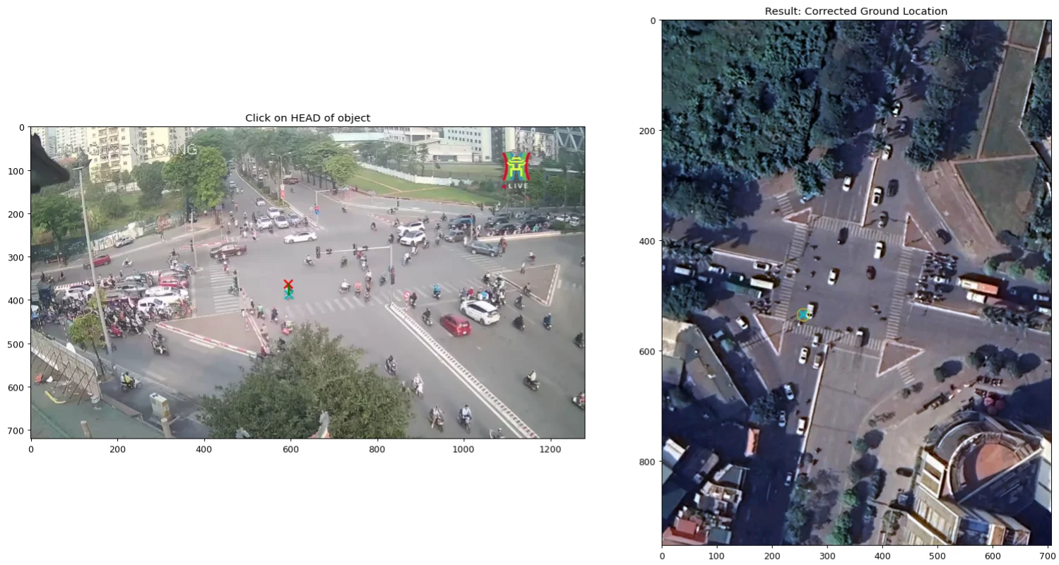
Clicking on a rider’s head (Red X) in CCTV now correctly resolves to their true ground position (Aqua X) in SAT, rather than the ghosted location.

Metric Scale and Layout Alignment

Two finishing steps complete the $G$ Projection.

Metric Scale: To convert pixel distances to meters, we pick two anchor points visible in the satellite image, measure the real-world geodetic distance using Google Earth, and define:

$$r_{ptm} = \frac{\| P_A - P_B \|_{SAT}}{D_{real}} \quad (\text{pixels/meter})$$

Block

For 119NH (119 Nguyen Hoang St., My Dinh, Hanoi), two island corners 41.13m apart measured 253.22 pixels on the satellite image, giving $r_{ptm} \approx 6.16$ px/m.

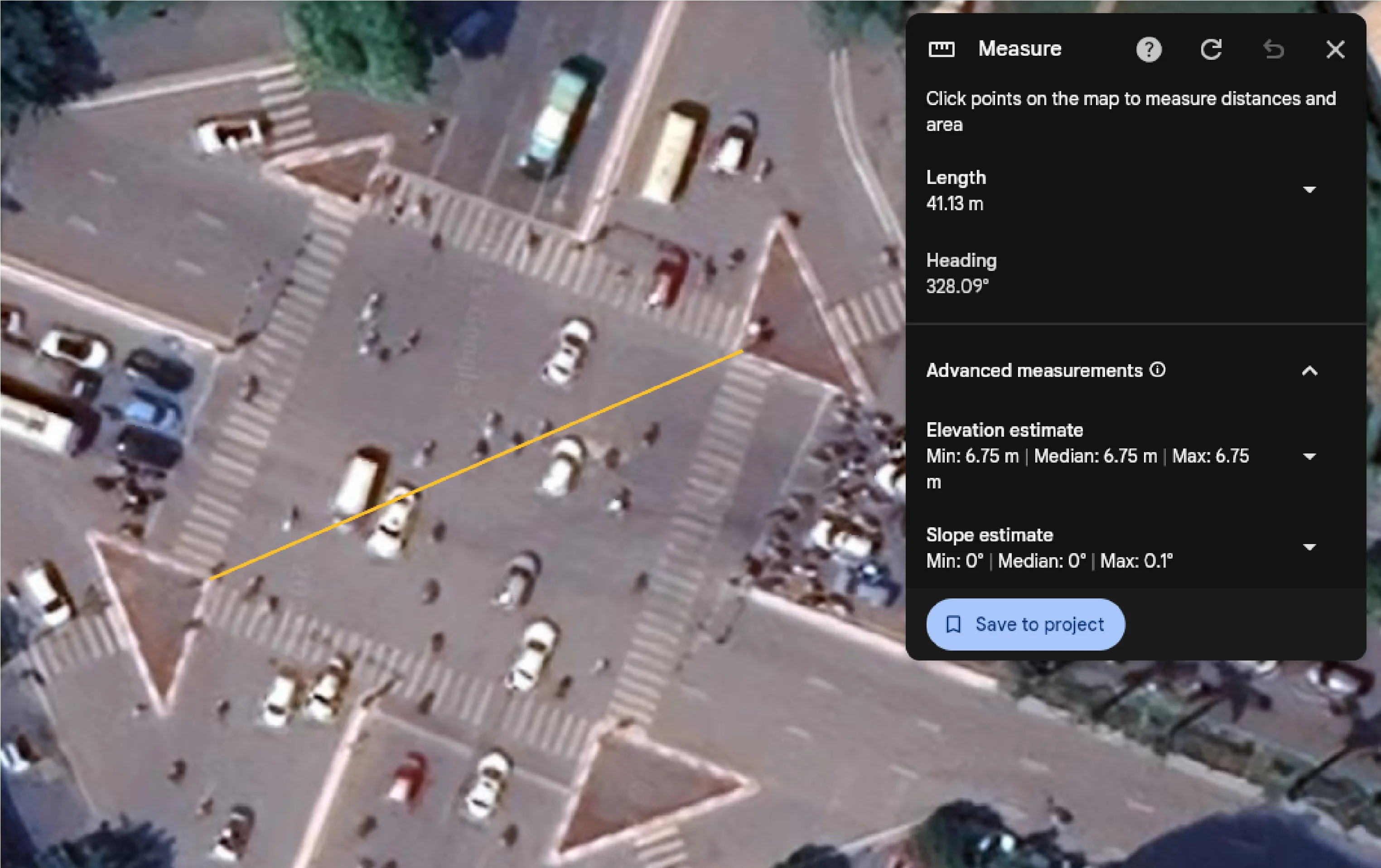
Real-world distance measurement between two road island corners via Google Earth, used to establish the pixel-to-meter ratio.

Layout Alignment: The optional SVG layout (road geometry drawn in Adobe Illustrator) lives in its own coordinate space. We compute the affine transform $A_{svg \rightarrow sat}$ that aligns it to the satellite image:

$$\left[ \begin{array}{c} x \\ y \end{array} \right]_{SAT} = \left[ \begin{array}{ccc} a_{11} & a_{12} & t_x \\ a_{21} & a_{22} & t_y \end{array} \right] \left[ \begin{array}{c} x \\ y \\ 1 \end{array} \right]_{LAYOUT}$$

Block

Using a minimum of 3 shared anchor points. This allows the SVG layers to be overlaid on the satellite image during visualization.

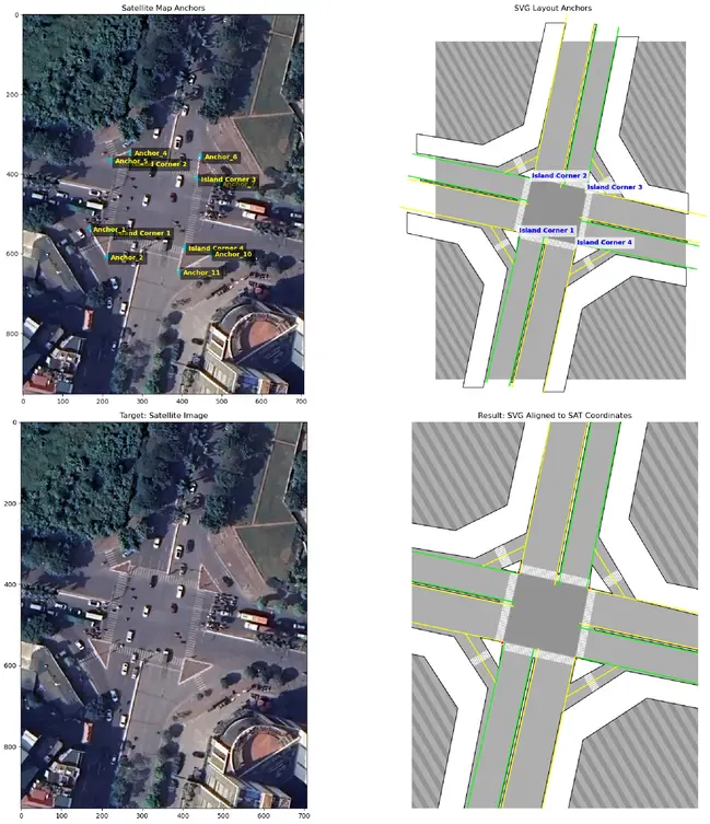
Anchors defined in both satellite (left) and SVG layout (right), and the resulting overlay (bottom).

All of this - the intrinsics, distortion coefficients, $H$, camera position and height, metric scale, FOV polygon, anchor set, and affine transform - is stored per-location as a single JSON file. That file is the $G$ Projection.

The X Engine

The $X$ Engine (Ten-step Engine) is the pipeline that uses the $G$ Projection to go from raw video to a 3D digital twin visualization. It takes three inputs in addition to the $G$ Projection: the CCTV footage, a prior dimension table $D_{prior}$ (assumed width, length, height per vehicle class in meters), and optionally the SVG $LAYOUT$.

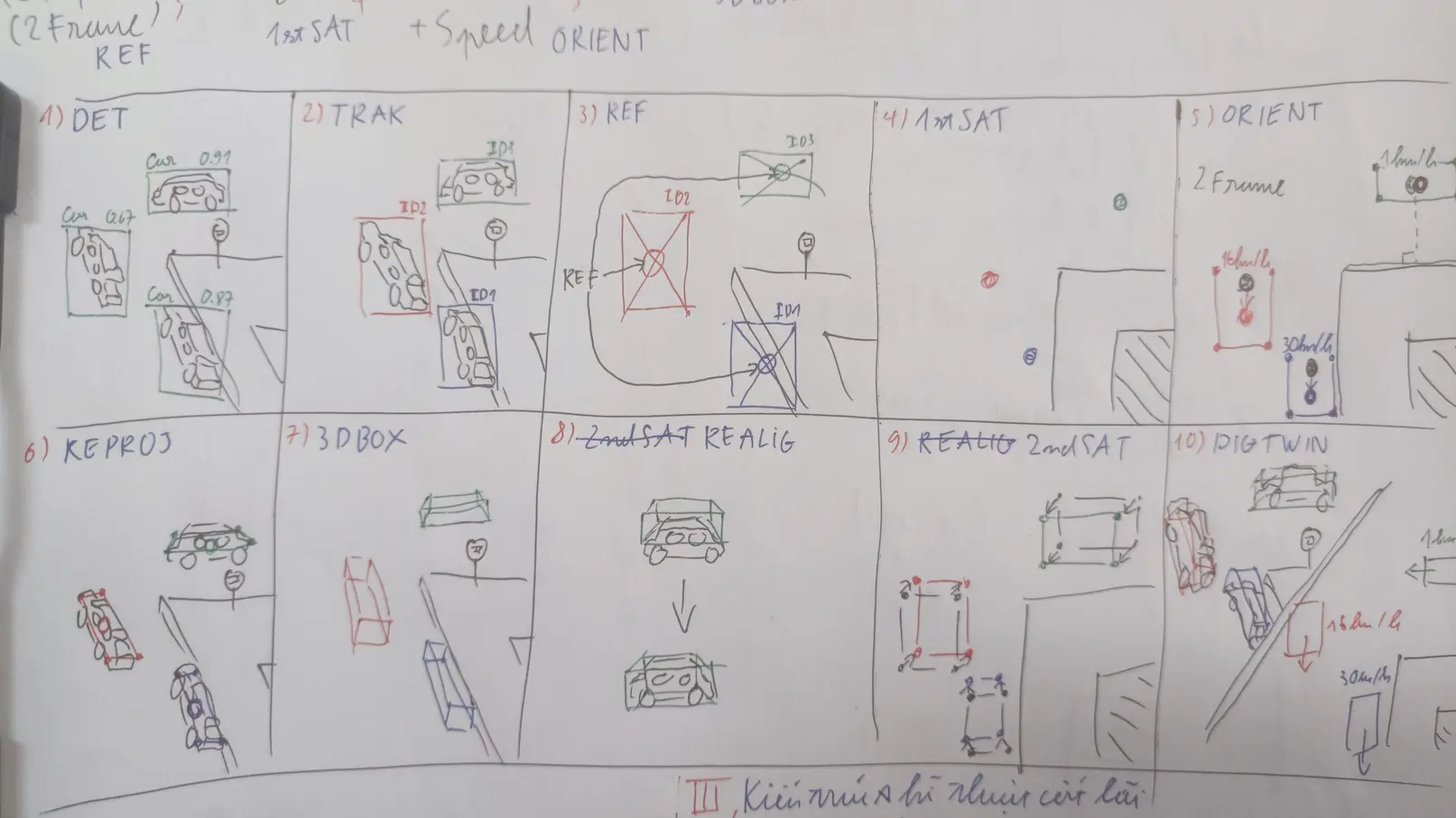
The $X$ Engine pipeline overview. Ten steps across three phases.

The pipeline is split into three phases.

Phase 1 - Perception

Step 1 - DET: Object detection. For the prototype, we fine-tuned YOLOv8-s (11.2M parameters) on the VisDrone dataset, with class adjustments to merge tricycle and awning-tricycle into a single three_wheeler class. Input size was set to 736px (a multiple of 32), close to the resolution of the HTVTraffic footage while keeping inference fast.

Training settled at mAP50 ≈ 0.43 and mAP50-95 ≈ 0.26. The F1 curve peaks at 0.47 with a confidence threshold of 0.210. The confusion matrix is candid: car and bus perform well, bicycle is essentially missed (74% classified as background), and motor, three_wheeler, truck, and van all have 35–55% false negative rates. The culprit is input resolution - small vehicles at 736px simply don’t have enough pixels to be resolved reliably.

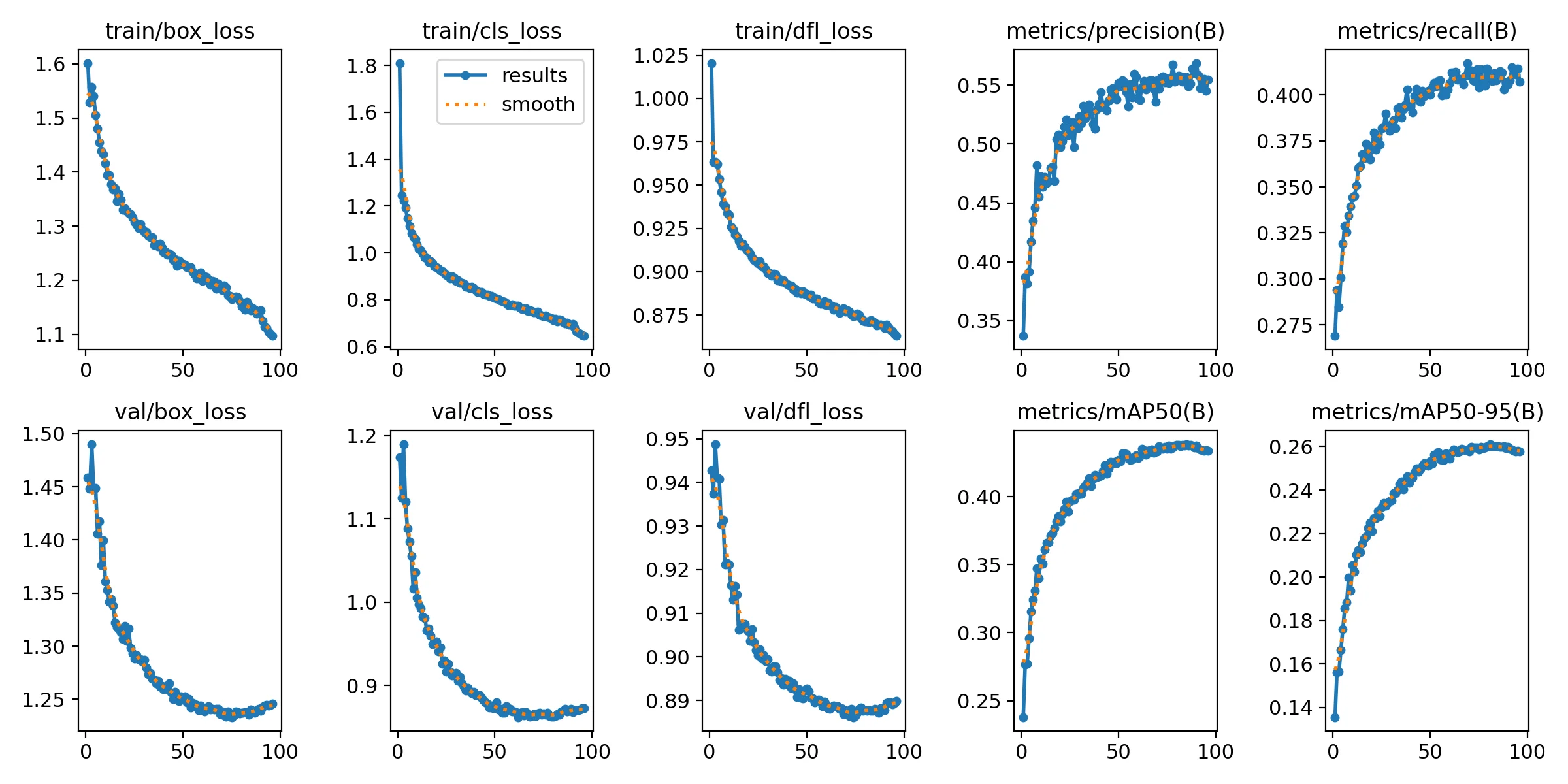
Loss and validation curves for the YOLOv8-s fine-tuning run on VisDrone. Convergence around epoch 80.

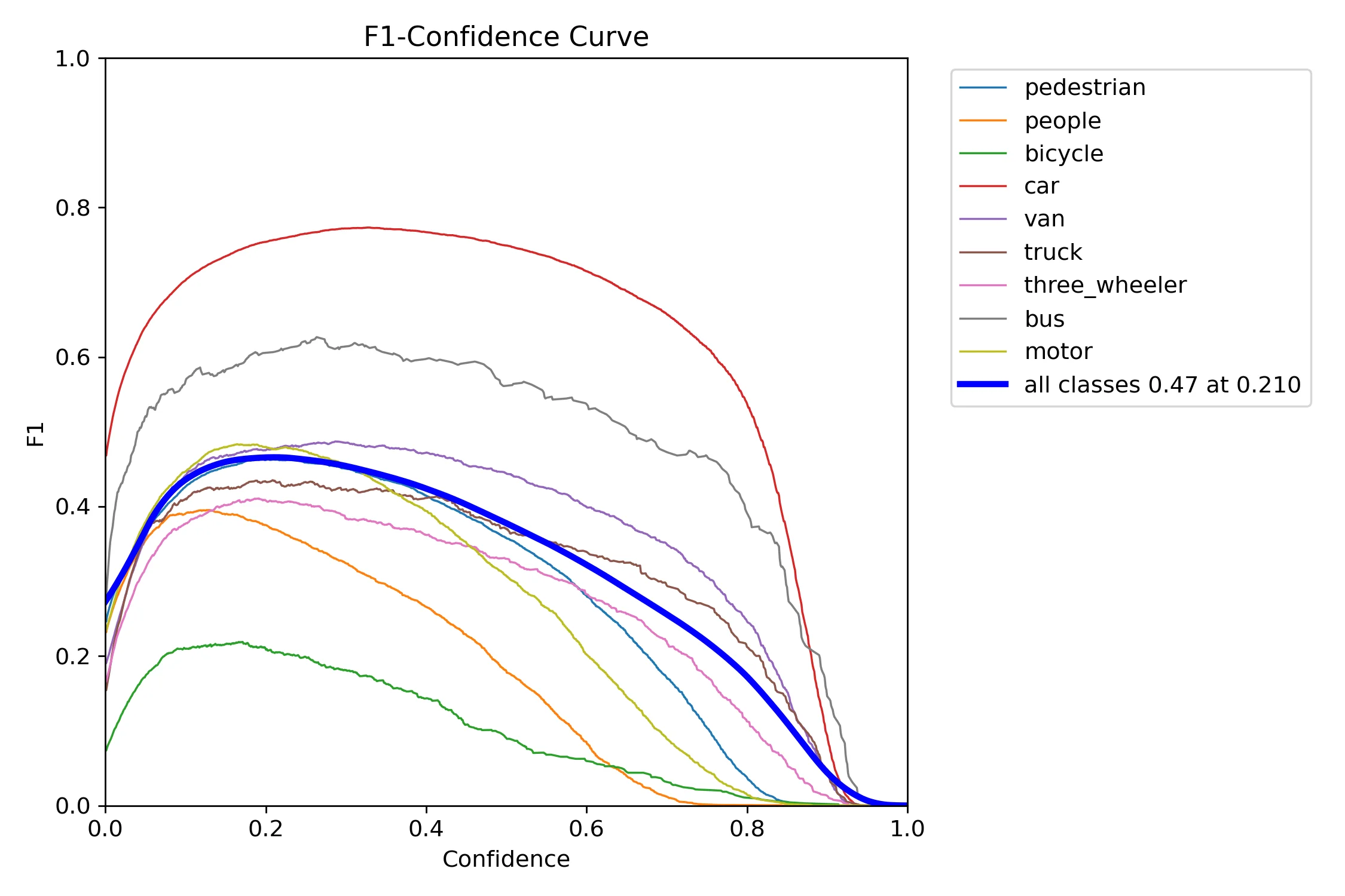
F1 curve by class. The model leans toward precision over recall, consistent with small-object detection difficulty.

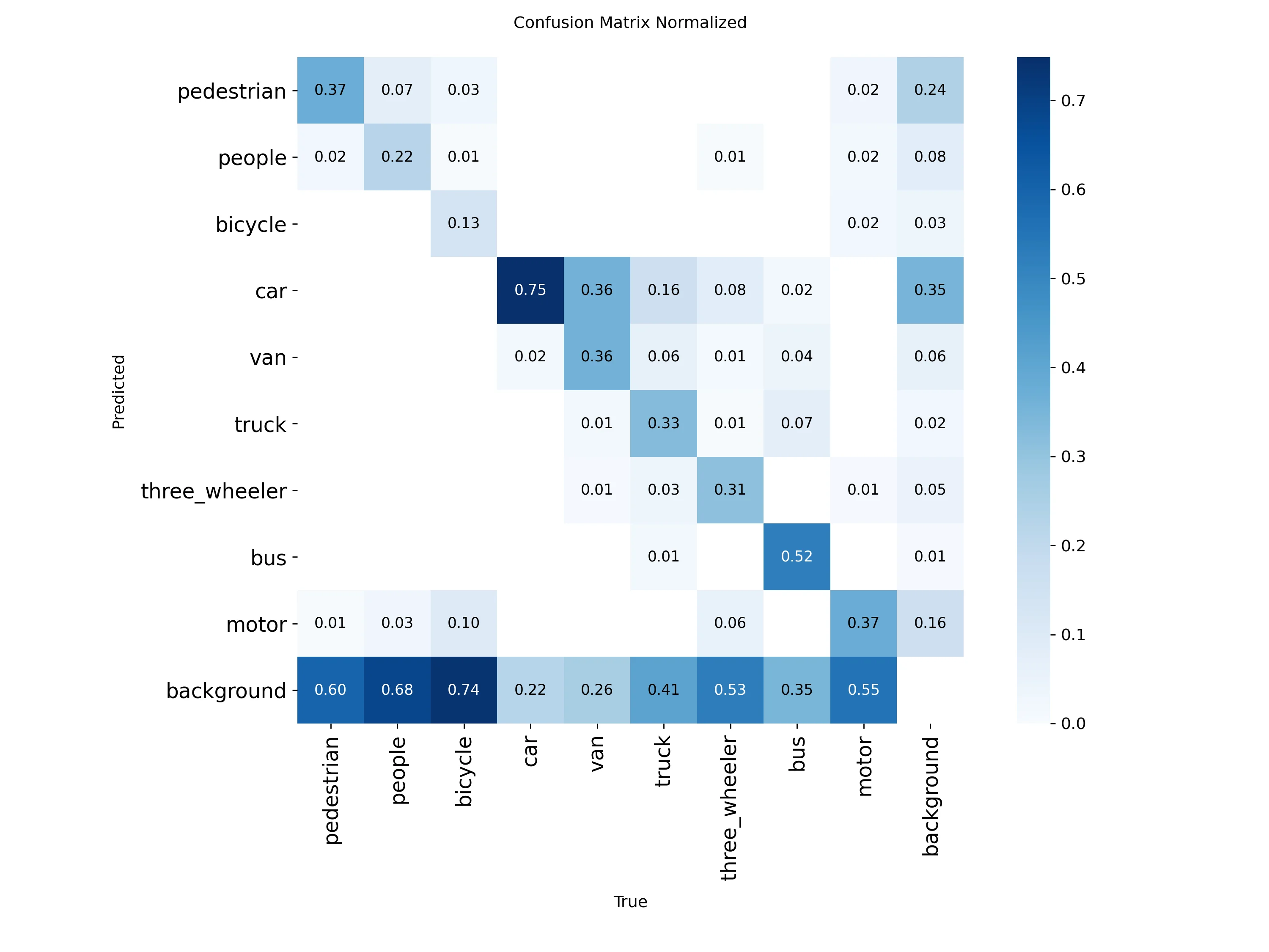
Normalized confusion matrix for the fine-tuned YOLOv8-s.

The inference arguments used for the prototype:

imgsz: 736
conf: 0.35
iou: 0.5
max_det: 600
agnostic_nms: false
half: true

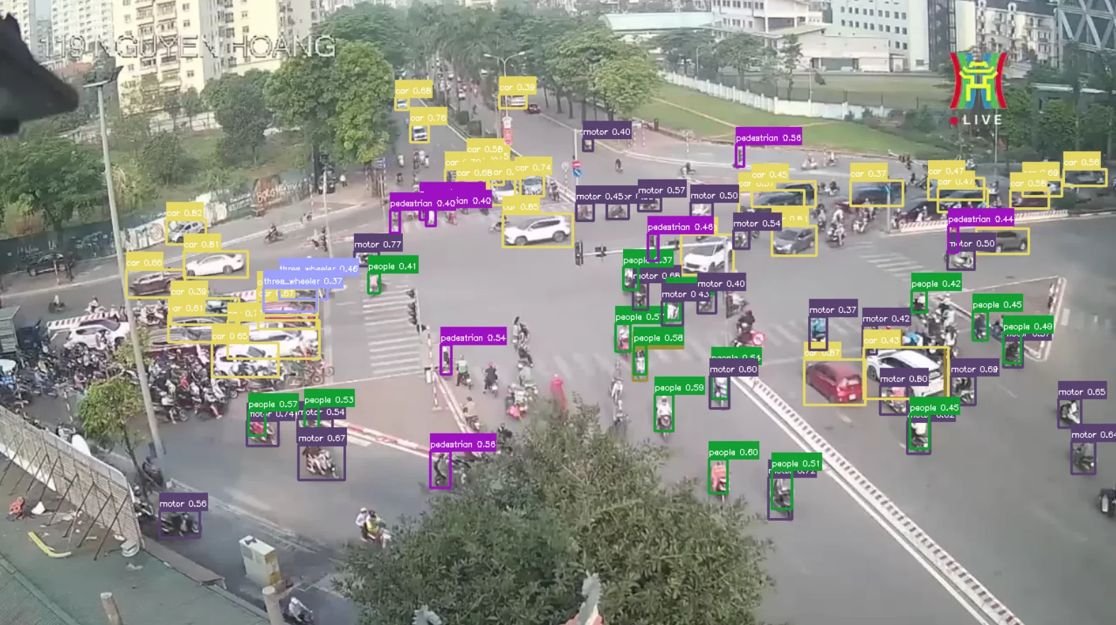
DET step output at 119NH.

Step 2 - TRAK: Multi-object multi-class tracking, using ByteTrack. ByteTrack’s main contribution is that it does not immediately discard low-confidence detections - instead, it runs a two-stage association cascade that first matches tracks to high-confidence detections, then tries to recover unmatched tracks using the low-confidence pool. This improves ID continuity in crowded scenes.

Formally, at frame $t$, the detection set is split by a threshold $\tau$:

$$\mathcal{D}_t^{\text{high}} = \{ d_i^t \mid s_i^t \ge \tau \}, \quad \mathcal{D}_t^{\text{low}} = \{ d_i^t \mid s_i^t < \tau \}$$

Block

Each track $k$ maintains a Kalman Filter state:

$$\mathbf{x}_k^t = \left[ \begin{array}{cccccccc} x & y & w & h & \dot{x} & \dot{y} & \dot{w} & \dot{h} \end{array} \right]^\top$$

Block

The association cascade first matches predicted tracks against $\mathcal{D}_t^{\text{high}}$ via Hungarian algorithm on IoU cost:

$$C_{k,i} = 1 - \text{IoU}(\hat{b}_k^t, b_i^t)$$

Block

Unmatched tracks then go through a second association against $\mathcal{D}_t^{\text{low}}$ using the same criterion. Tracks unmatched for more than $ T_{lost} $ frames are removed. Unmatched high-confidence detections initialize new tracks.

ByteTrack arguments for the prototype:

tracker_type: bytetrack
track_high_thresh: 0.25
track_low_thresh: 0.1
new_track_thresh: 0.25
track_buffer: 30
match_thresh: 0.8
fuse_score: true

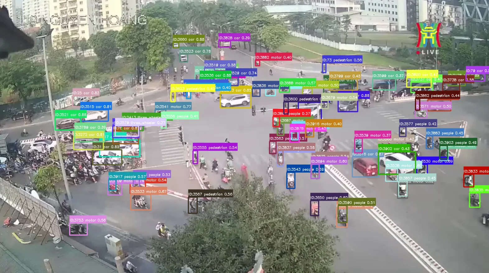
TRAK step output at 119NH. Each road user has a persistent ID.

Step 3 - REF: From each tracked bounding box $b_k^t = (x_k^t, y_k^t, w_k^t, h_k^t)$, we derive a reference point representing the object. The center of the box is used:

$$\phi(b_k^t) = \left[ \begin{array}{c} x_k^t + w_k^t/2 \\ y_k^t + h_k^t/2 \end{array} \right] = p_k^t$$

Block

This gives us a tracked point set:

$$\mathcal{P}_t = \left( \text{ID}_k,\ c_k,\ p_k^t \right)_{k=1}^{K_t}$$

Block

Ideally, the reference point would be the ground contact point of each vehicle - 3D-Net uses the center of the bottom edge. We use the box center because the bottom edge can be occluded or cut by the ROI boundary, making it less stable in practice. The tradeoff is a projection height error we compensate for in the next step.

Phase 2 - Projection & Geometry

Step 4 - 1stSAT: The first use of $G_1$. We project the reference points from CCTV space into satellite space. Since we are using the box center rather than the ground contact point, we approximate the projection height as half of the class prior height:

$$\mathcal{P}_{t}^{\text{1stSAT}} = G_1\!\left( \mathcal{P}_{t},\ h = h_{c_k}^{\text{prior}}/2 \right)$$

Block

This gives us $\mathbf{s}_k^t = (x_k^t, y_k^t)_{SAT}$ - the inferred satellite coordinates for each tracked road user.

Step 5 - ORIENT: With objects located on the satellite map, we estimate their heading and speed by looking at how their position changes across frames.

The displacement vector in satellite space is:

$$\mathbf{d}_k^t = \mathbf{s}_k^t - \mathbf{s}_k^{t - \Delta t}$$

Block

We convert the Euclidean magnitude to meters using $r_{ptm}$, then to speed:

$$v_k^t = \frac{D_{metric}}{\Delta t / \text{FPS}} \quad (\text{m/s})$$

Block

If $D_{metric} < 0.3\text{m}$, the object is classified as stationary and heading defaults to whatever the road geometry dictates via the $LAYOUT$ layers. Otherwise, the raw heading is:

$$\theta_{raw}^t = \text{arctan2}(\Delta y, \Delta x) \cdot \frac{180}{\pi}$$

Block

Raw headings are inherently noisy. We apply three stabilization layers:

Adaptive EMA: The smoothing factor scales with speed - faster objects produce more reliable displacement vectors. The EMA factor:

$$\alpha^t = \text{clip}\!\left( \alpha_{min} + \frac{v_k^t}{v_{ref}} (\alpha_{max} - \alpha_{min}),\ \alpha_{min},\ \alpha_{max} \right)$$

Block

Smoothed heading update:

$$\theta_{k}^t = \theta_{k}^{t-1} + \alpha^t \cdot \text{wrap}(\theta_{raw}^t - \theta_{k}^{t-1})$$

Block

with $\alpha_{min} = 0.05$ and $\alpha_{max} = 0.4$.

Jitter Bubble: If the satellite coordinates remain within a 0.6m radius for 8 consecutive frames, the movement is treated as detector jitter and heading is frozen.

Cosine Gating: Angular changes below 10° are fully accepted; above 30° are rejected as physically impossible. Between these thresholds, the update weight is linearly dampened.

With a stabilized heading $\theta_k^t$, the floor-box for each object is constructed in satellite space using $D_{prior}$ dimensions scaled by $r_{ptm}$:

$$l_{px} = \frac{L \cdot r_{ptm}}{2}, \quad w_{px} = \frac{W \cdot r_{ptm}}{2}$$

Block

The four corners of the floor-box are:

$$\mathbf{c}_j = \mathbf{s}_k^t + \mathbf{R}(\theta_k^t) \cdot \mathbf{m}_j$$

Block

where the rotation matrix is $\mathbf{R}(\theta_k^t) = \left[ \begin{array}{cc} \cos\theta & -\sin\theta \ \sin\theta & \cos\theta \end{array} \right]$ and the four unrotated corner offsets are:

$$\mathbf{m}_1 = \left[ \begin{array}{c} l_{px} \\ w_{px} \end{array} \right], \\ \mathbf{m}_2 = \left[ \begin{array}{c} l_{px} \\ -w_{px} \end{array} \right], \\ \mathbf{m}_3 = \left[ \begin{array}{c} -l_{px} \\ -w_{px} \end{array} \right], \\ \mathbf{m}_4 = \left[ \begin{array}{c} -l_{px} \\ w_{px} \end{array} \right]$$

Block

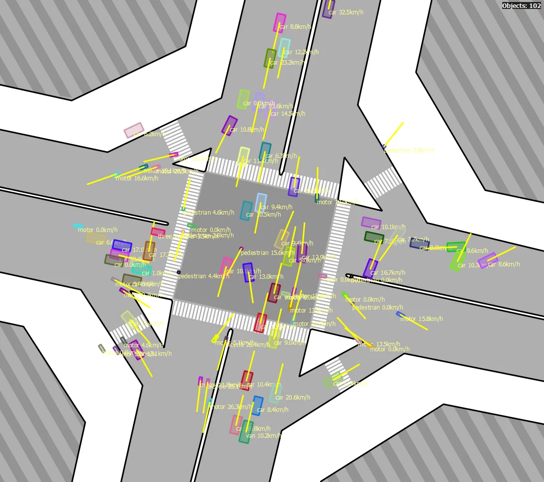
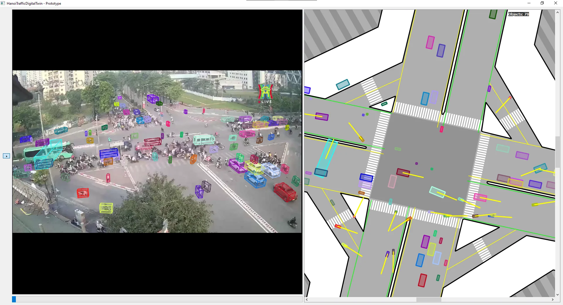
ORIENT step output. Floor boxes on the satellite map, with heading arrows (yellow) and speed labels (km/h). Stationary vehicles without reliable heading data are defaulted by the LAYOUT guidelines.

Step 6 - REPROJ: The four floor-box corners $\{\mathbf{c}_j\}_{j=1}^4$ are on the ground plane, so we project them back to CCTV using $G_2$ at $h = 0$:

$$\mathbf{u}_j^{\text{bottom}} = G_2(\mathbf{c}_j, h=0)$$

Block

This gives us the perspective-distorted quadrilateral footprint of each vehicle on the ground in the camera image.

Phase 3 - Reconstruction

Step 7 - 3DBOX: Having the 4 bottom vertices in CCTV space, we now compute the 4 top vertices by projecting the same satellite corners back at the object’s prior height $h = h_{c_k}^{\text{prior}}$:

$$\mathbf{u}_j^{\text{top}} = G_2(\mathbf{c}_j,\ h_{c_k}^{\text{prior}})$$

Block

The complete 3D bounding box is the union of bottom and top vertices:

$$\mathcal{B}_{3D} = \{ \mathbf{u}_1^{\text{bottom}}, \dots, \mathbf{u}_4^{\text{bottom}},\ \mathbf{u}_1^{\text{top}}, \dots, \mathbf{u}_4^{\text{top}} \}$$

Block

This extrudes the 2D floor rectangle vertically in perspective, producing a wireframe cuboid that respects the scene geometry.

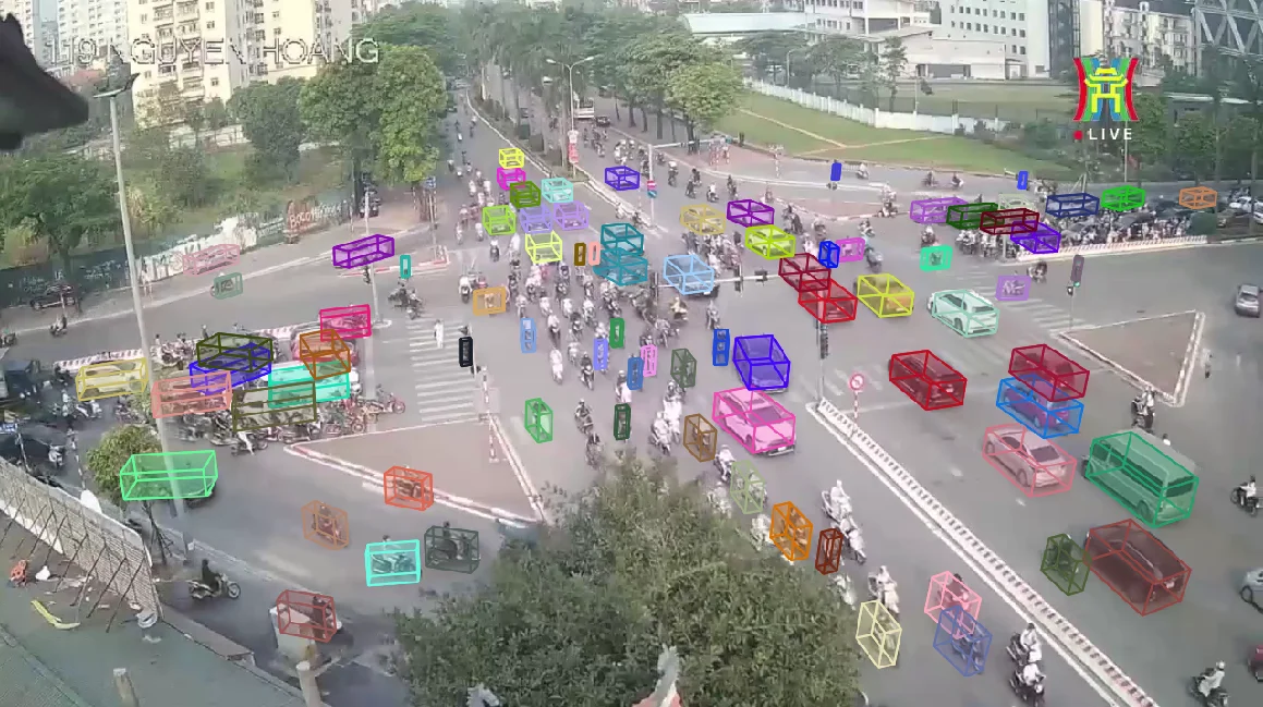
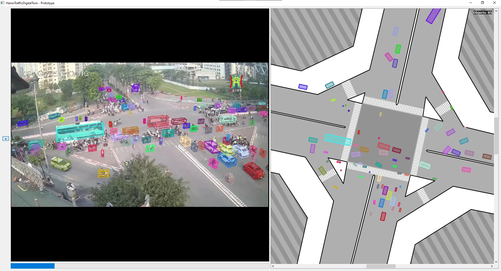
3DBOX step output at 119NH.

Steps 8 & 9 - REALIG & 2ndSAT: These steps are theoretically defined but not implemented in the current prototype. REALIG would automatically refine the 3D box fit in CCTV - $D_{prior}$ gives us a plausible starting box, but there is no guarantee the prior dimensions match the actual vehicle. 2ndSAT would then correct the satellite floor box accordingly. These remain open engineering problems, and the reasoning for not pursuing them yet is straightforward: given that DET is already the bottleneck producing noisy boxes, it would be premature to invest heavily in refining a 3D reconstruction built on unreliable input. The priority needs to be detection quality first.

Step 10 - DIGT: The final visualization - a synchronized side-by-side view of the CCTV panel (with 3D boxes) and the satellite panel (with speed and heading-aware floor boxes). This is the digital twin display.

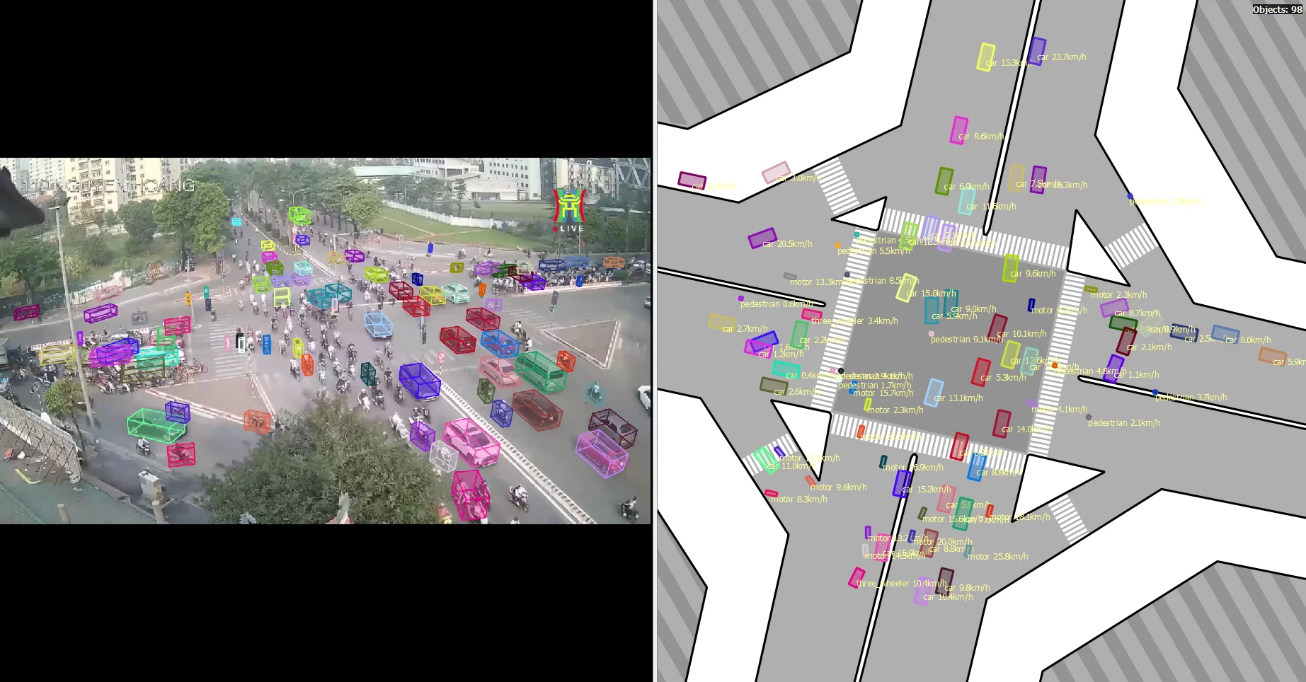
The DIGT step: the complete digital twin view for location 119NH.

TrafficLab 3D - The Application

The prototype (originally named HTDT - HanoiTrafficDigitalTwin) has since been refactored into TrafficLab 3D, a general-purpose desktop application with a proper calibration workflow and no hardcoded location assumptions.

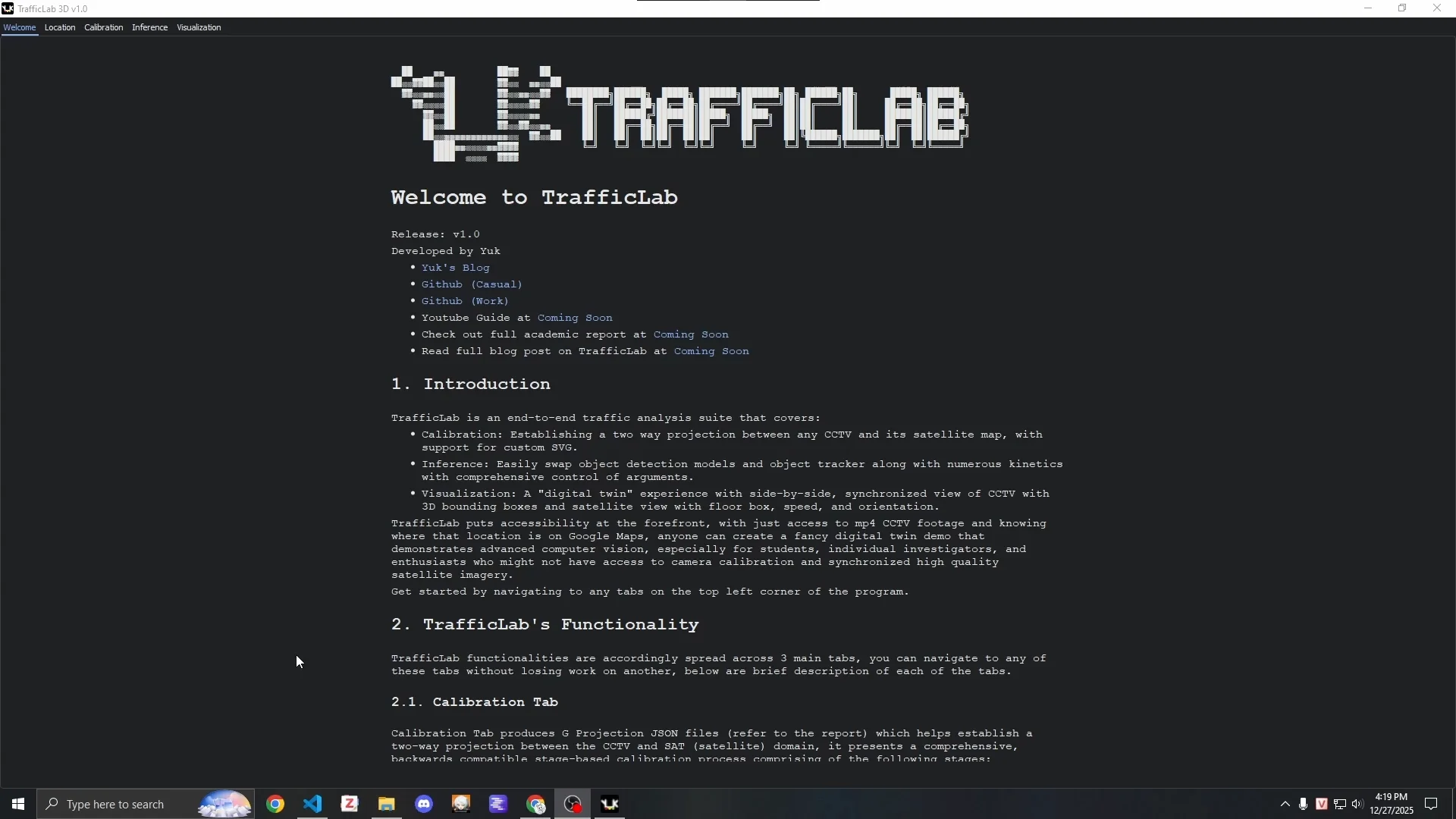
TrafficLab 3D welcome screen.

The application is organized into three tabs, accessible from the top-left corner without losing work on other tabs.

Calibration Tab: A stage-based GUI that walks through the entire $G$ Projection construction process described above - undistortion, homography anchor placement, parallax subject selection, SVG alignment, ROI definition, and final validation. Each stage has a visual feedback mechanism. The final validation stage lets you test 2D-to-3D conversion interactively before saving.

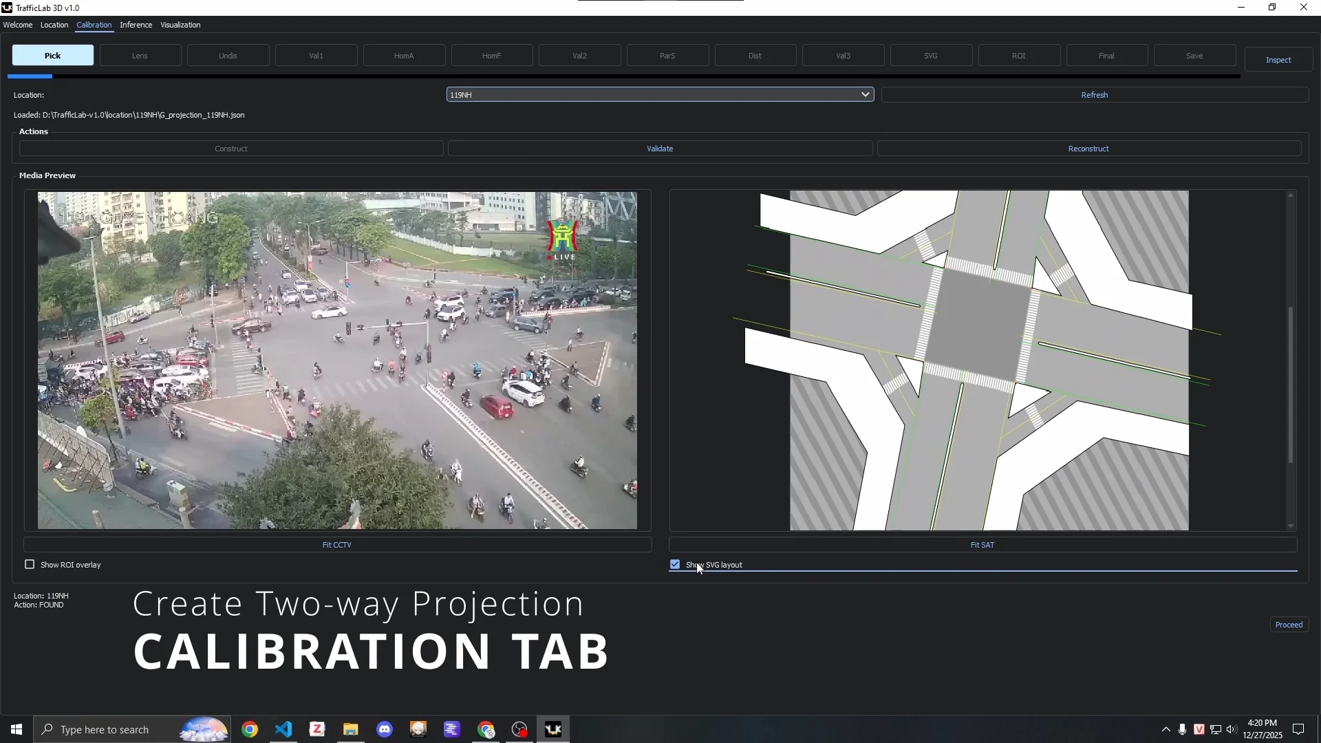
The Calibration Tab at the start of the pipeline.

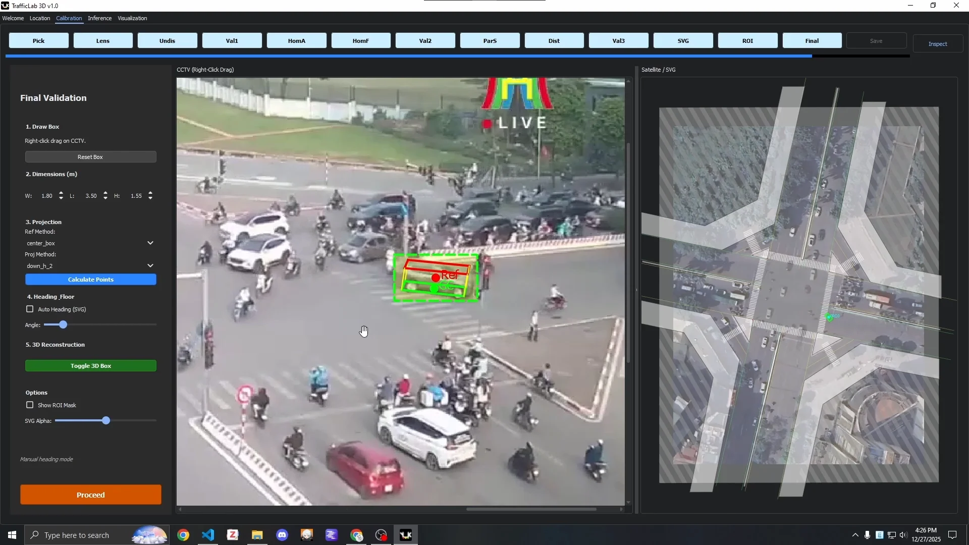
The final calibration validation stage: testing 3D box construction before saving the G Projection JSON.

Inference Tab: Controls model and tracker selection, and manages inference runs. Arguments are set through inference_config.yaml and prior_dimensions.json. Inference output is saved as .json.gz compressed files - precomputing the pipeline outputs means the visualization engine does not need to run detection and tracking in real time.

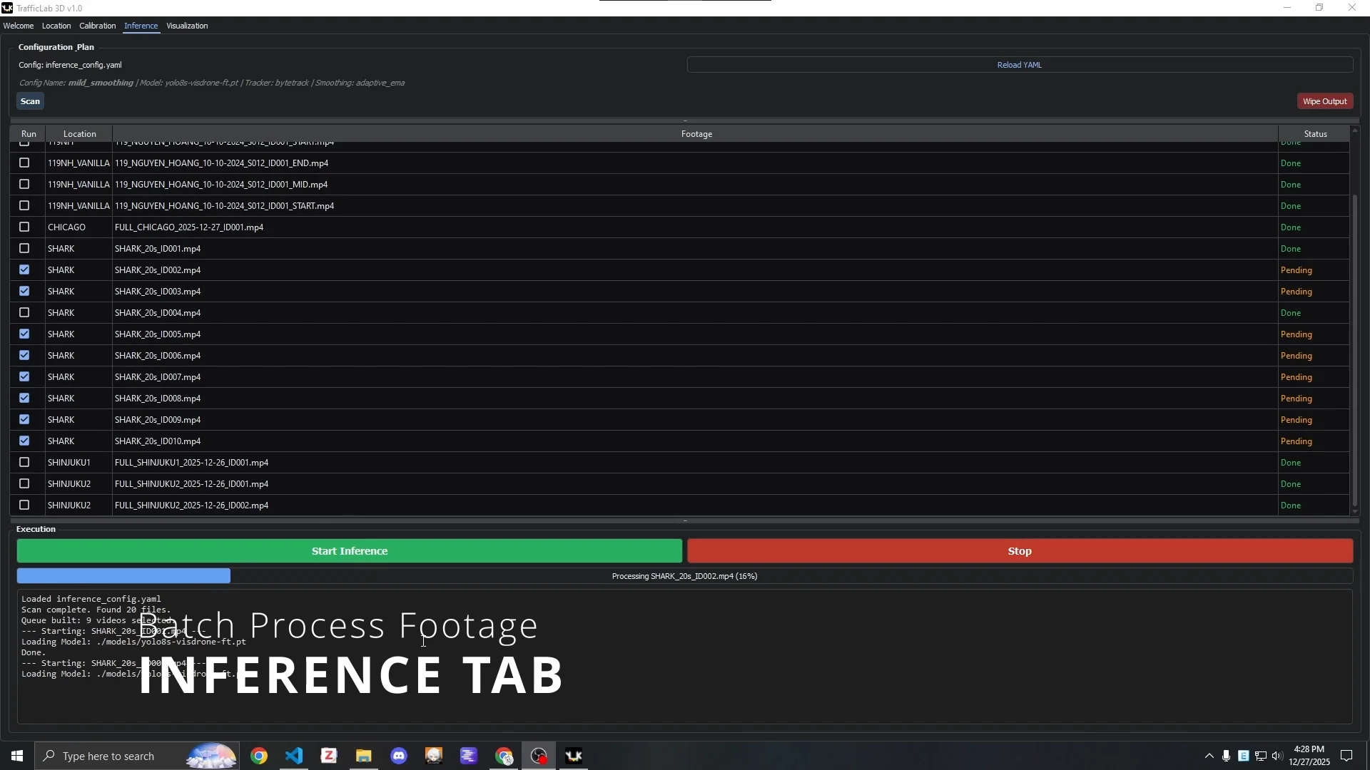
The Inference Tab, tracking all produced output files.

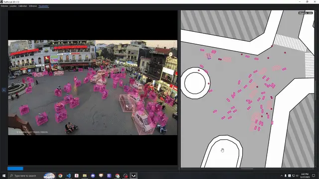
Visualization Tab: Loads a .json.gz result file and runs the synchronized CCTV + SAT visualization with full keyboard shortcut support, toggleable overlays, and collapsible panels.

The Visualization Tab: side-by-side CCTV (with 3D boxes) and satellite (with floor boxes) view.

The file structure for each location follows:

TrafficLab-3D/
├── location/
│   └── {location_code}/
│       ├── footage/
│       │   └── *.mp4
│       ├── G_projection_{location_code}.json
│       ├── cctv_{location_code}.png
│       └── sat_{location_code}.png
├── models/
│   └── *.pt
├── output/
│   └── model-{model}_tracker-{tracker}/
│       └── {config}/
│           └── {location_code}/
│               └── *.json.gz
├── inference_config.yaml
├── prior_dimensions.json
└── main.py

Getting started requires only a conda environment and main.py:

conda env create -f environment.yml
python main.py

Pre-constructed $G$ Projections for several locations, fine-tuned YOLO model checkpoints, and a ready-to-visualize .json.gz output file are available on the project’s Google Drive.

Qualitative Analysis

We ran the pipeline across six Hanoi locations and one high-quality reference clip, and the patterns in the failures are fairly diagnostic.

119NH (119 Nguyen Hoang, My Dinh, Hanoi):

The cyan bus has an ill-fitted 3D box. Bitrate compression makes most motorcycles invisible to the detector. The far white bus gets a nonsensical box from detection noise.

Detection noise caused the same bus to undergo an impossible rotation between frames despite extensive smoothing. The lower-right lane shows guideline-assisted orientation working correctly. The adjacent lane, further from the guidelines, does not.

107LHP (107 Le Hong Phong, Ba Dinh):

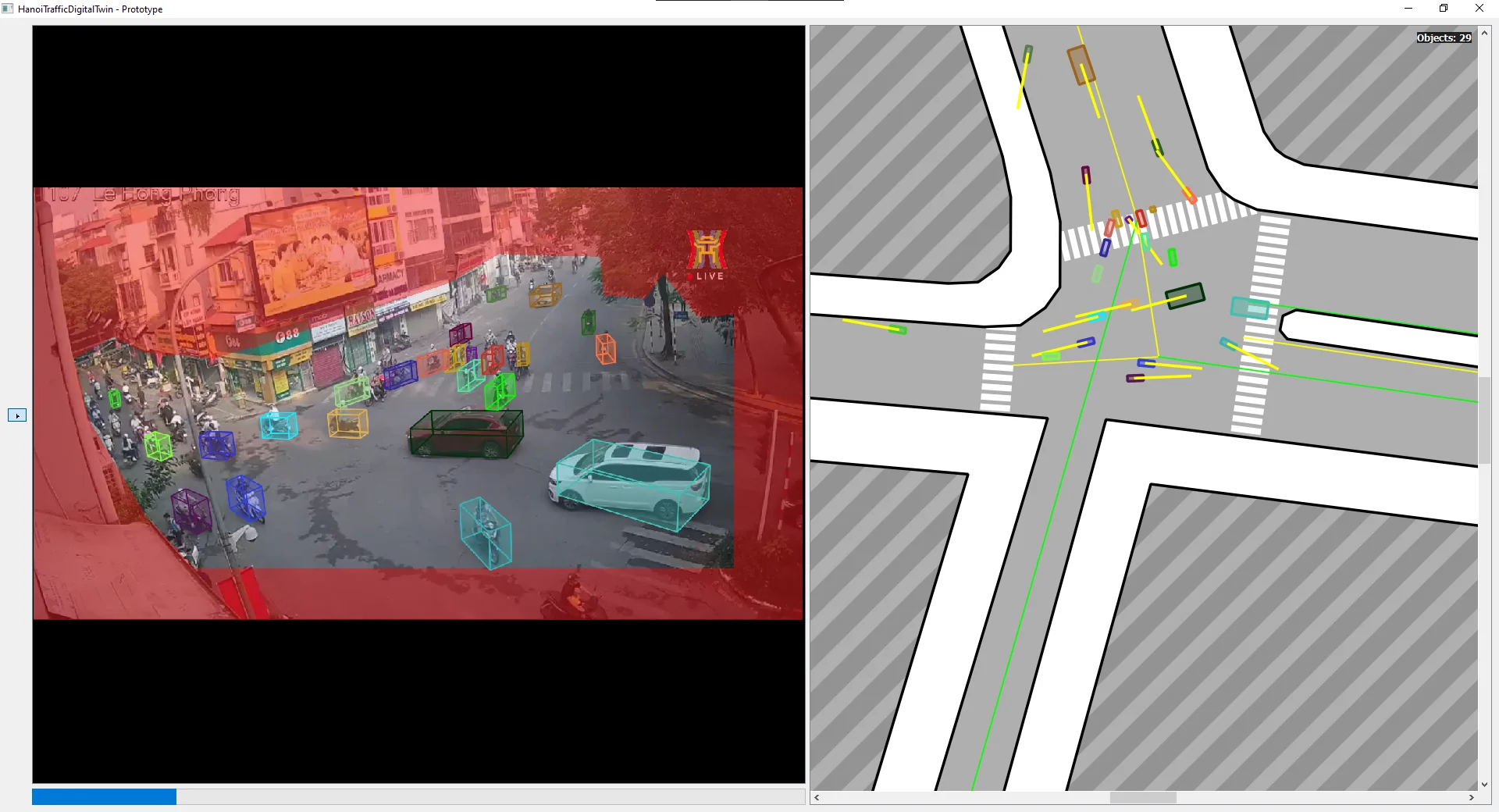
White SUV on the left has bad default orientation - it was moving slowly near the ROI boundary. The alleyway on the left side has severe compression artifacts; the detector misses essentially everything in that zone.

150OCD (150 O Cho Dua, Dong Da):

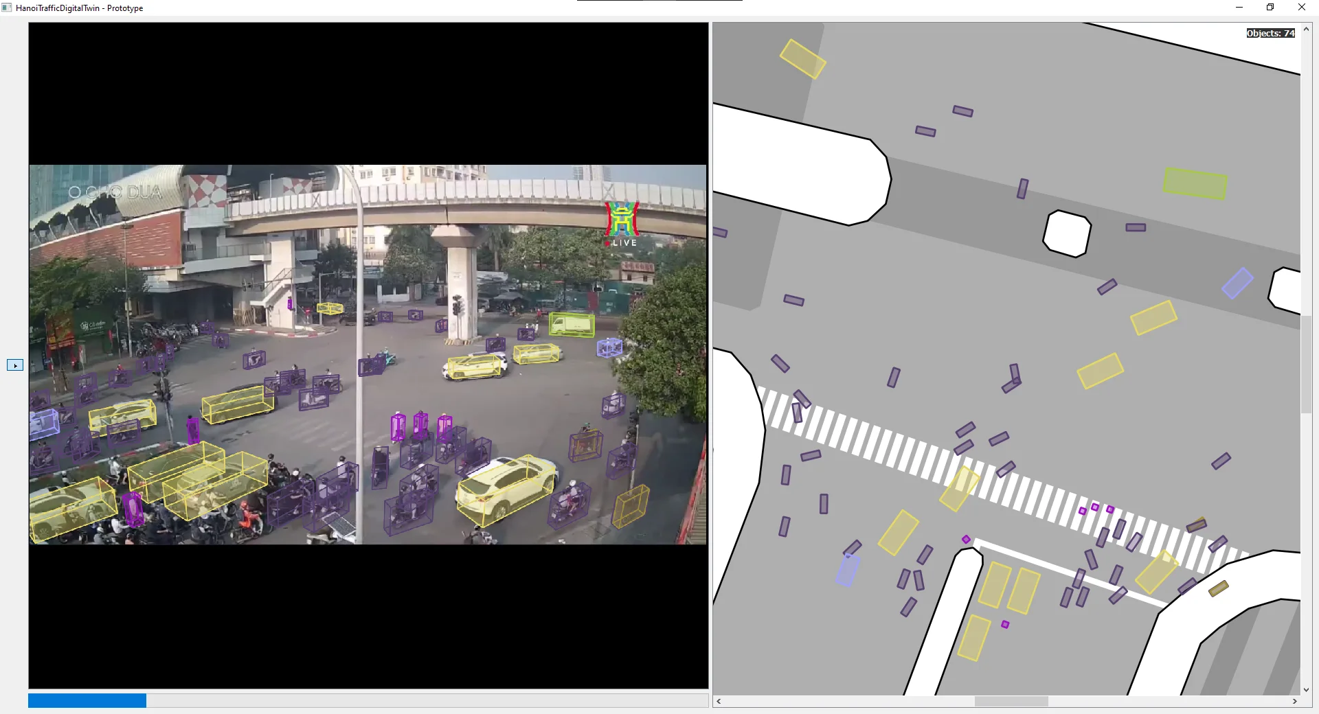
Three motorcycle riders in the center of frame are mistaken for pedestrians due to camera angle and occlusion. Two more near the right edge are classified as three-wheelers.

45NLB (45 Nguyen Luong Bang, Dong Da):

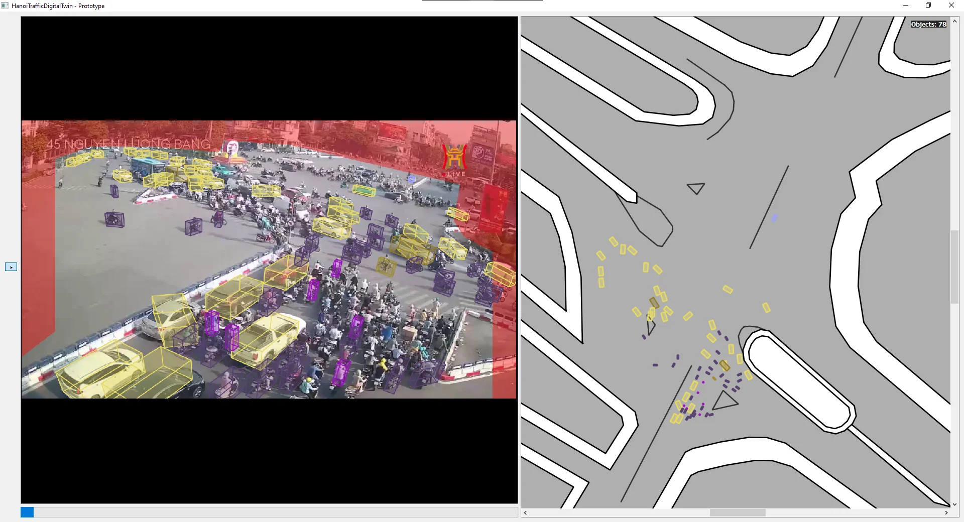
The most complex flat intersection in the dataset. Also the worst compression. These two properties compound.

71NT (71 Nguyen Trai, Thanh Xuan):

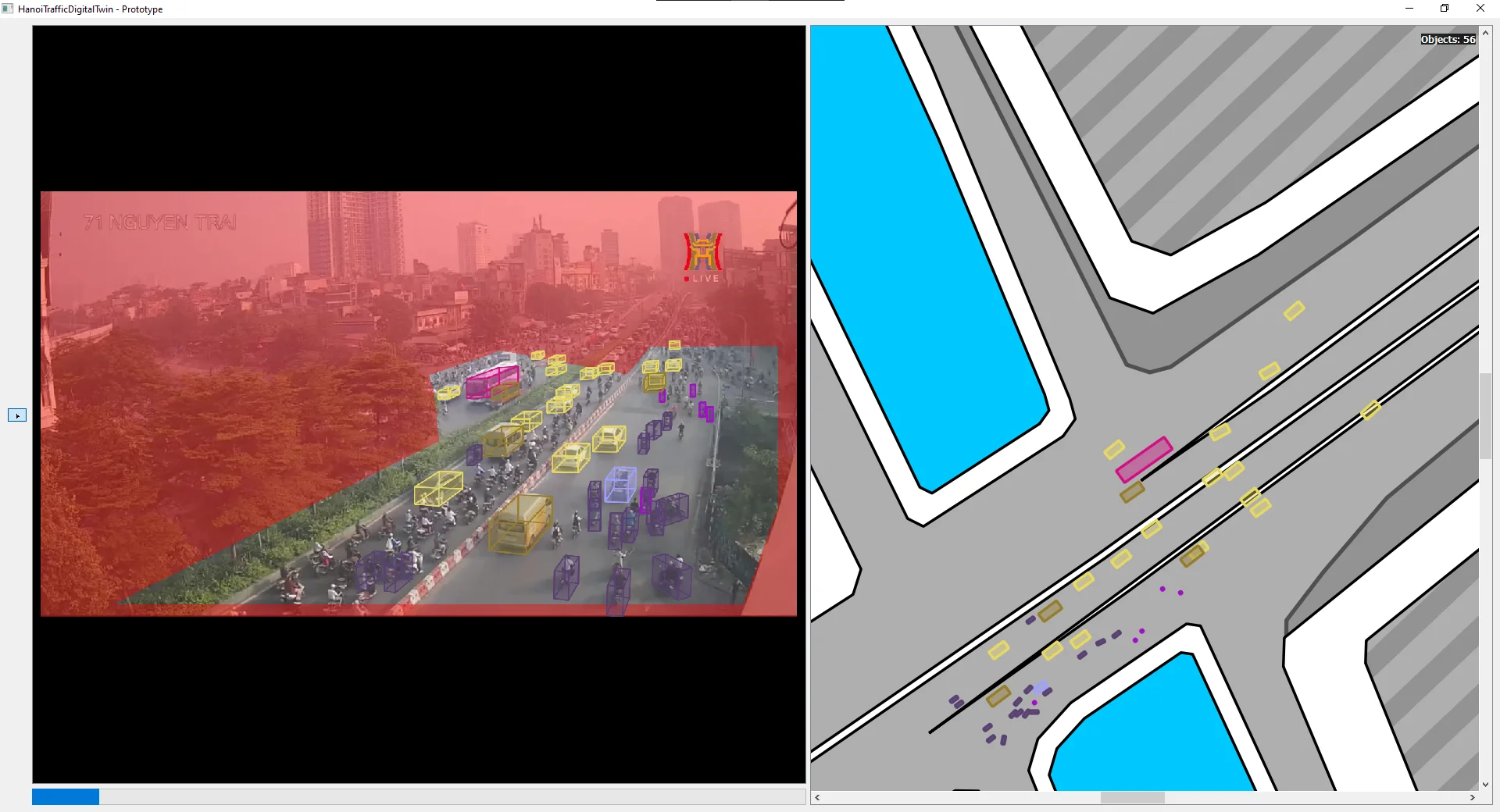
The ROI had to cut out a large portion of the camera’s FOV because part of the road is sloped - the $G$ Projection is valid only for flat planar surfaces. You can see exactly where it fails: further along the slope, the floor boxes in SAT start overlapping barricades, which is physically impossible.

SHARK (7 Dinh Tien Hoang, Hoan Kiem - the “Shark Jaw” building, since demolished):

This is the only high-resolution reference clip in the set, originally 4K, downscaled cleanly without compression artifacts.

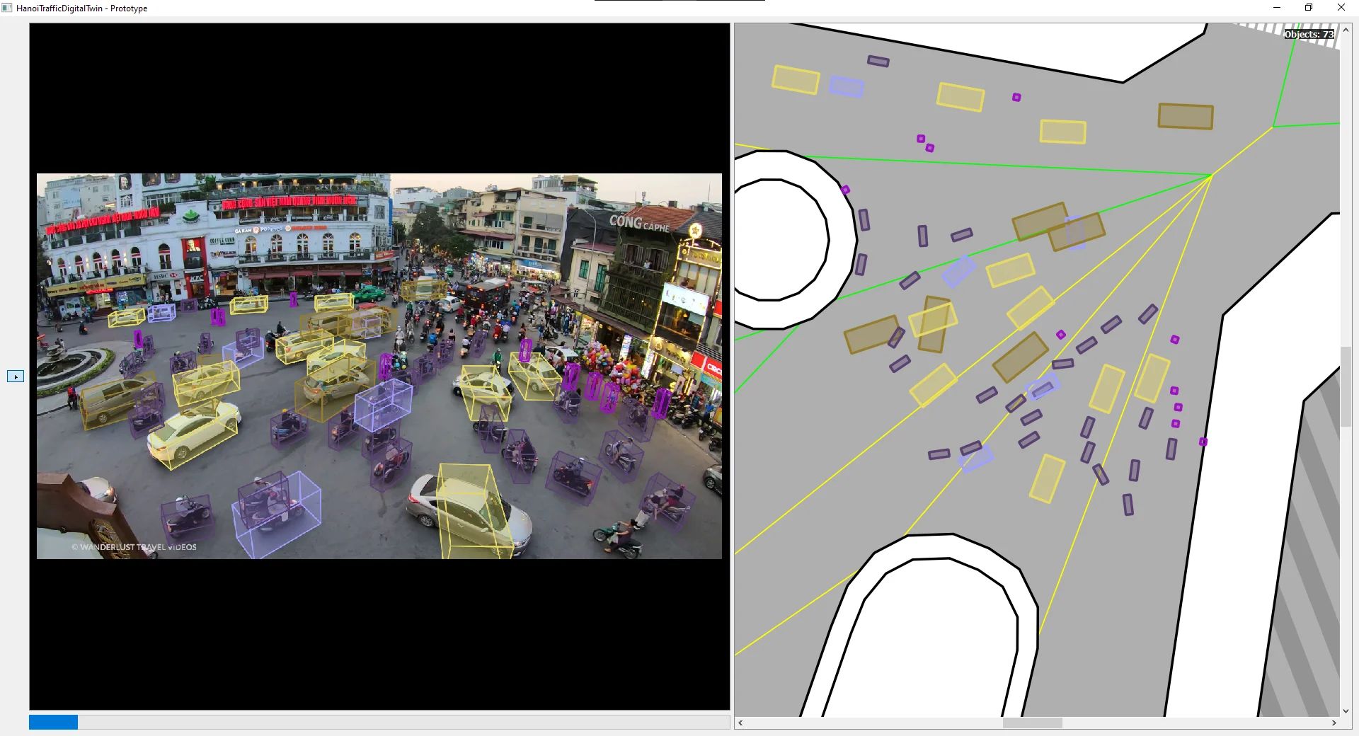
Clean footage, noticeably better results. Still shows the limits of guideline-based orientation for non-standard Hanoi infrastructure - slow or stationary vehicles at unusual angles get wrong defaults.

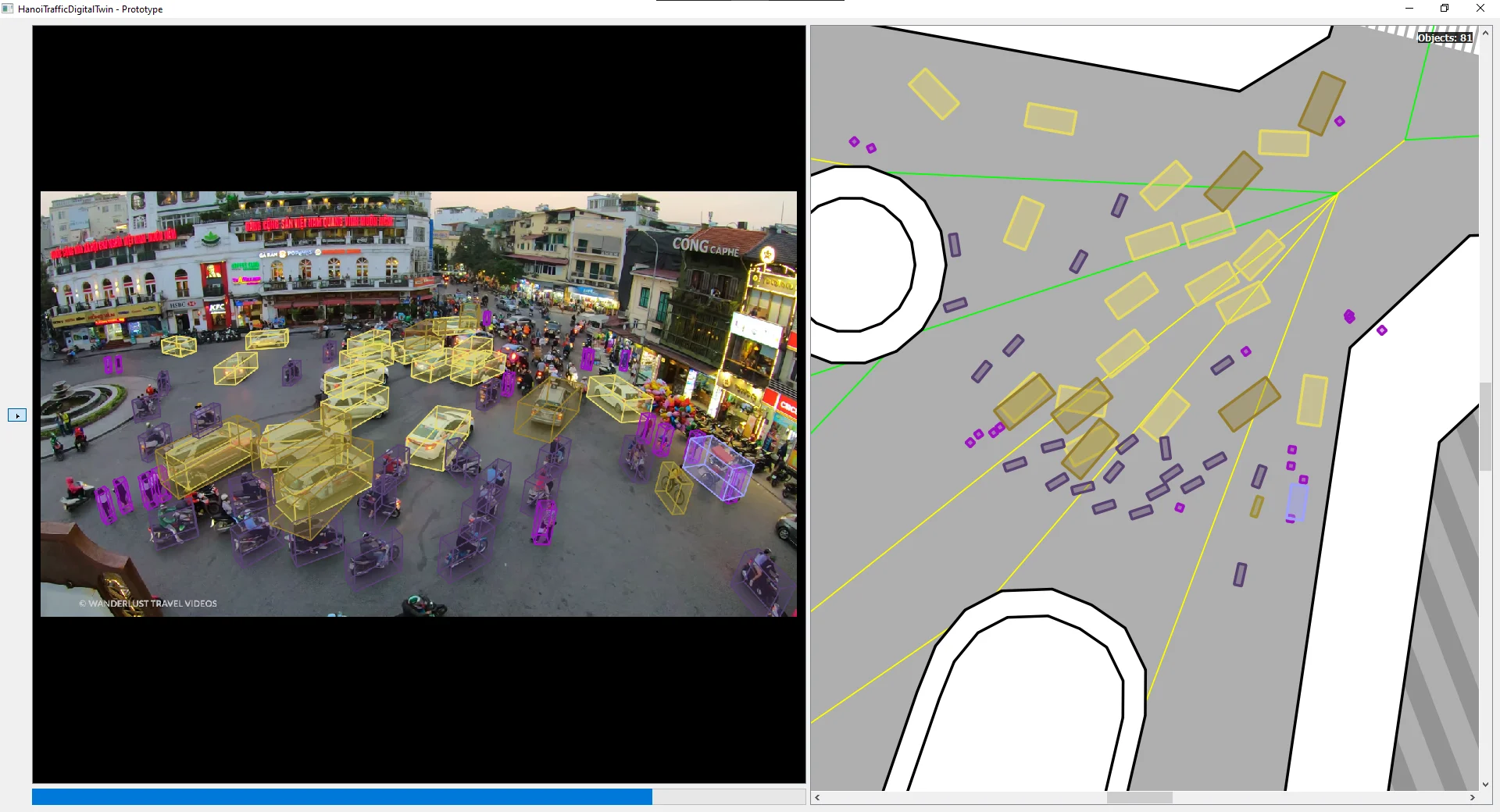
The car/van confusion from the VisDrone training data is visible here most clearly: double boxes, ID switches, and nonsensical satellite behavior from misclassified vehicles.

The pattern is consistent across all locations. When the detector produces clean output, the geometric pipeline works. When it does not - because of low bitrate, small object size, or class confusion - everything downstream degrades accordingly. The $G$ Projection and $X$ Engine are not the bottleneck. Step 1 is.

What Remains Open

There are three things that the current prototype does not solve.

Detection quality on low-bitrate footage. The HTVTraffic dataset is real, publicly sourced Hanoi traffic video, and it is 720p with heavy compression artifacts from network streaming. Motorcycles at this resolution with this much JPEG-style blocking are genuinely hard to detect. Fine-tuning on VisDrone helped with class coverage but not with resolution. The SHARK clip demonstrates that the rest of the pipeline is capable - the bottleneck is the input quality, not the geometry.

Steps 8 and 9. REALIG and 2ndSAT are the unimplemented refinement steps. $D_{prior}$ gives us a reasonable first estimate for 3D box dimensions, but the actual vehicles in the scene have actual dimensions that may differ significantly. Correcting the 3D box fit automatically - using the 2D detection box as a constraint - is the next logical step, but it depends on having a reliable 2D detection to constrain against. Solving detection first makes sense.

Non-flat geometry. The $G$ Projection is defined for a flat ground plane. The ROI mechanism handles sloped terrain by exclusion, but there is no current mechanism for handling multi-level infrastructure (overpasses, underpasses) within a single camera view. Extending the framework to handle multiple plane hypotheses or piecewise planar scenes is a longer-term problem.

Closing Remarks

TrafficLab 3D is available at duy-phamduc68/TrafficLab-3D with pre-built environments, pre-calibrated locations, and a detailed setup guide. The long-term vision is city-wide - automatic calibration, continuous detector improvement, and eventually a system sufficient for high-fidelity simulation and reinforcement learning. For now, it is a working proof-of-concept that anyone with a video clip and a Google Maps screenshot can run on their own machine.

The core geometric ideas - parallax ray triangulation, the bidirectional $G$ Projection, and the floor-box extrusion pipeline - are, I think, the transferable parts of this work. They hold up even when everything else is noisy.

References

• Rezaei, M., Azarmi, M., & Mir, F. M. P. (2023). 3D-Net: Monocular 3D Object Recognition for Traffic Monitoring. Expert Systems with Applications, 227, 120253. Link
• AISKYEYE Team, Tianjin University. VisDrone-DET2019: The Vision Meets Drone Object Detection in Image Challenge Results. Link
• Data source: HTV Youtube Channel (Hanoi Radio & Television). Link
• Data source: Wanderlust Travel Videos Youtube Channel. Link